Modeling Preliminaries - Programming for Data Science (Fall 2025)

import pandas as pd
import seaborn as sns
from scipy import stats
import numpy as np
from sklearn.model_selection import train_test_split
from sklearn.naive_bayes import GaussianNB
from sklearn.metrics import confusion_matrix, classification_report, roc_auc_score 
import matplotlib.pyplot as plt

sns.set_theme(palette='colorblind')

Identity matrices¶

D = 4
np.eye(D)

array([[1., 0., 0., 0.],
       [0., 1., 0., 0.],
       [0., 0., 1., 0.],
       [0., 0., 0., 1.]])

3*np.eye(D)

array([[3., 0., 0., 0.],
       [0., 3., 0., 0.],
       [0., 0., 3., 0.],
       [0., 0., 0., 3.]])

Gaussian Distribution¶

The Gaussian also known as normal distribution. It can be univariate or multivariate](#dist:multivariategaussian). In one dimension it is shaped like a bell curve and in two dimensions it is like hill. It has two parameters, the mean that shifts its location(in one dim along the axis or in either/both directions in two dims) and the scale changes the shape. In one dimenion the scale is the variance and controls the width. In two dimensions the scale is the covariance matrix, its diagonal controls the width and height and the off diagonals control the skew(angle)

Univariate Gaussian¶

in one dimension is like:

P(x) = \frac{1}{\sigma\sqrt{2\pi}} e^{-\frac{1}{2}\left(\frac{x-\mu}{\sigma}\right)^2}

(1)

where:

$x$ is the scalar random variable
$\sigma^2$ is the variance (the scale parameter )
$\mu$ is the mean (the location parameter)

x = np.linspace(-10, 10, 1000)
var = 1
mu = 0
plt.plot(x, stats.norm.pdf(x, loc=mu, scale=var), 
         label=r'$\mu=0, \sigma=1$', linewidth=2)
plt.title(f'Univariate Gaussian with mean={mu} and var={var} ')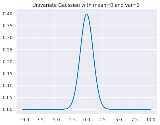

The mean parameter changes the location of the distribution

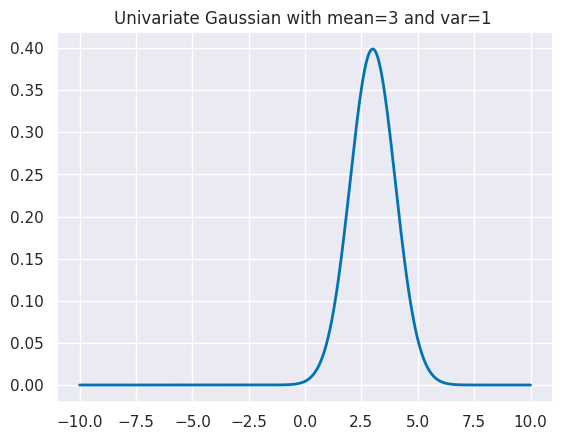
and the scale controls how wide it is.

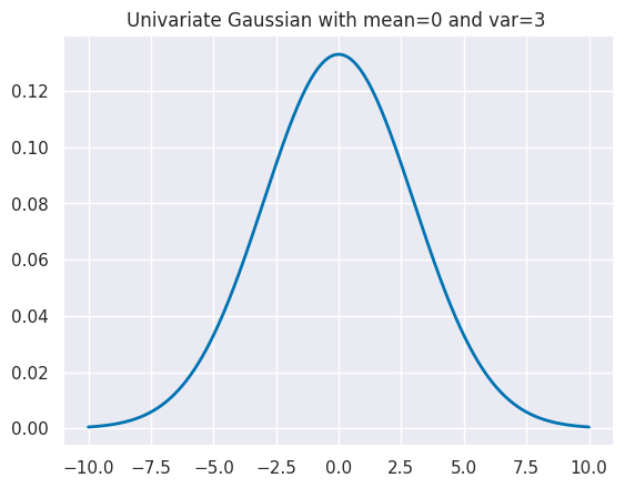
Multivariate Gaussian¶

For a vector random variable it is written:

P(\mathbf{x}) = \frac{1}{\sqrt{(2\pi)^k|\boldsymbol{\Sigma}|}} \exp\left(-\frac{1}{2}(\mathbf{x}-\boldsymbol{\mu})^T\boldsymbol{\Sigma}^{-1}(\mathbf{x}-\boldsymbol{\mu})\right)

(2)

where:

$\mathbf{x}$ is the vector random variable
$\boldsymbol{\Sigma}$ is the covariance matrix
$\boldsymbol{\mu}$ is the vector mean
$^T$ is the transpose operator

In 2D we can plot the density with a contour plot:

mu = np.array([0, 0])  # mean vector
cov = np.array([[1, 0],    # covariance matrix
                [0, 1]])

# Create a grid of points
x = np.linspace(-4, 4, 100)
y = np.linspace(-4, 4, 100)
X, Y = np.meshgrid(x, y)

# Stack X and Y to create position array
pos = np.dstack((X, Y))

# Create multivariate normal distribution
mvn = stats.multivariate_normal(mu, cov)

# Evaluate PDF at grid points
Z = mvn.pdf(pos)

# Create contour plot
contours = plt.contour(X, Y, Z, levels=10, colors='blue')
plt.contourf(X, Y, Z, levels=20, alpha=0.6, cmap='Blues')
plt.colorbar(label='Probability Density')
plt.title(f'MVN with mean={mu} and cov={cov} ')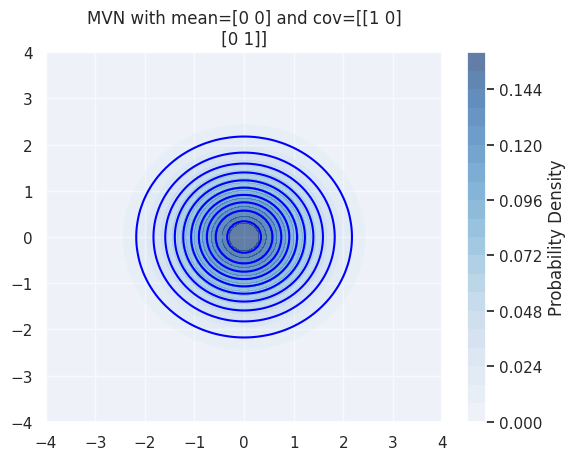

The mean still controls the location

mu = np.array([2, 1])  # mean vector

# Create multivariate normal distribution
mvn = stats.multivariate_normal(mu, cov)

# Evaluate PDF at grid points
Z = mvn.pdf(pos)

# Create contour plot
contours = plt.contour(X, Y, Z, levels=10, colors='blue')
plt.contourf(X, Y, Z, levels=20, alpha=0.6, cmap='Blues')
plt.colorbar(label='Probability Density')
plt.title(f'MVN with mean={mu} and cov={cov} ')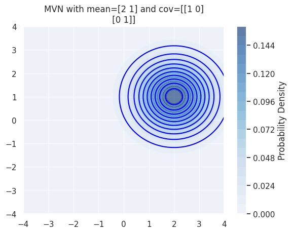

The main diagonal of the covariance control controls the width and height

mu = np.array([0, 0])  # mean vector
cov = np.array([[2, 0],    # covariance matrix
                [0, .5]])

# Create multivariate normal distribution
mvn = stats.multivariate_normal(mu, cov)

# Evaluate PDF at grid points
Z = mvn.pdf(pos)

# Create contour plot
contours = plt.contour(X, Y, Z, levels=10, colors='blue')
plt.contourf(X, Y, Z, levels=20, alpha=0.6, cmap='Blues')
plt.colorbar(label='Probability Density')
plt.title(f'MVN with mean={mu} and cov={cov} ')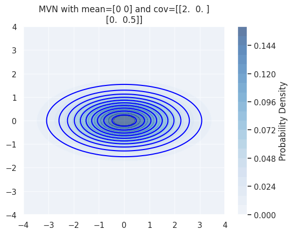

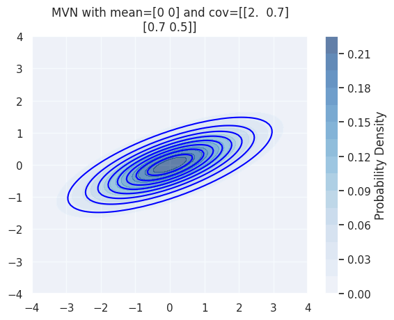
The off diagonal elements of the covariance control controls the angle or skew

mu = np.array([0, 0])  # mean vector
cov = np.array([[2, .7],    # covariance matrix
                [.7, .5]])

# Create multivariate normal distribution
mvn = stats.multivariate_normal(mu, cov)

# Evaluate PDF at grid points
Z = mvn.pdf(pos)

# Create contour plot
contours = plt.contour(X, Y, Z, levels=10, colors='blue')
plt.contourf(X, Y, Z, levels=20, alpha=0.6, cmap='Blues')
plt.colorbar(label='Probability Density')
plt.title(f'MVN with mean={mu} and cov={cov} ')