Evaluating ML Algorithms - Programming for Data Science (Fall 2025)

This week we are going to start learning about machine learning.

We are going to do this by looking at how to tell if machine learning has worked.

This is because:

you have to check if one worked after you build one
if you do not check carefully, it might only sometimes work
gives you a chance to learn only evaluation instead of evaluation + an ML task

What is a Machine Learning Algorithm?¶

First, what is an Algorithm?

An algorithm is a set of ordered steps to complete a task.

Note that when people outside of CS talk about algorithms that impact people’s lives these are often not written directly by people anymore. They are often the result of machine learning.

One way to think of machine learning is that, people write an algorithm for how to write an algorithm that solves a problem based on data. This often comes in the form of a statitistical model of some sort.

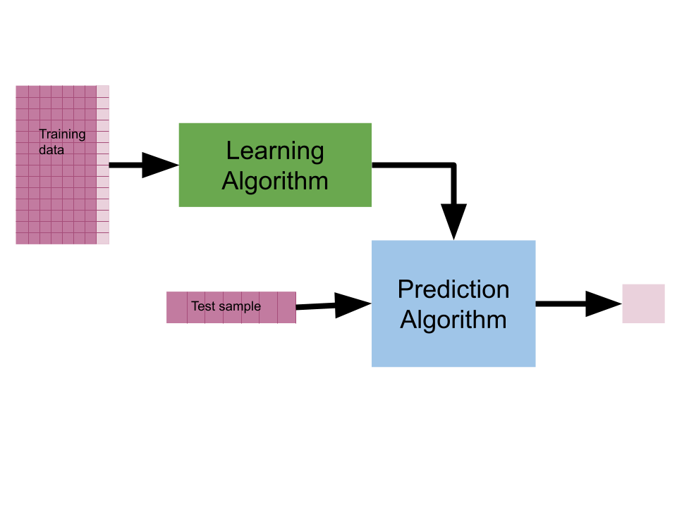
Ml overview: training data goes into the learning algorithm, which outputs the prediction algorithm. the prediciton algorithm takes a sampleand outputs a prediction

More precisly, people write a learning algorithm that finds the best parameters that precisely specify the prediction algorithm to work for the specific problem. The learning algorithm is given example data (typically features and a target)

If this is confusing...

A very simple example of this basic template is that the equation for a line:

y = mx +b

(1)

$m$ and $b$ are parameters
$x$ is the inputs, for features
$y$ is the output, or target

The learning algorithm would take in training data $(x,y)^D$ , that is $D$ distinct $(x,y)$ pairs. The prediction algorithm would take in one $x$ and return a prediction for the value of $y$ , typically called $\hat{y}$

We will return to this more, but in case it helps.

When we do machine learning, this can also be called:

data mining
pattern recognition
modeling

because we are looking for patterns in the data and typically then planning to use those patterns to make predictions or automate a task.

Each of these terms does have slightly different meanings and usage, but sometimes they’re used close to exchangeably.

How can we tell if ML is working?¶

If we knew the answer that the learning algorithm was supposed to find, we would just write the algorithm and we would not need the learning agorithm at all.

This means, in real^[1] problems, that we cannot directly check if it is correct.

Instead, we measure the performance of the prediction algorithm, to determine if the learning algorithm worked.

ML researchers, who develop new learning algorithms, evaluate the performance of the learning algoritm more generally, by applying it to many datasets and seeing if it works on all of them. Then we say the learning algorithm is good.

More often though, in real problems, we are interested in what is called model evaluation, or checking if the specific model we learned for this specific problem is good.

Replicating the COMPAS Audit¶

We are going to replicate the audit of the COMPAS algorithm by journalists at Propublica.

Why COMPAS?¶

Propublica started the COMPAS Debate with the article angwin2016machine. With their article, they also released details of their methodology and their data and code. This presents a real data set that can be used for research on how data is used in a criminal justice setting without researchers having to perform their own requests for information, so it has been used and reused a lot of times.

Propublica COMPAS Data¶

The dataset consists of COMPAS scores assigned to defendants over two years 2013-2014 in Broward County, Florida, it was released by Propublica in a GitHub Repository. These scores are determined by a proprietary algorithm designed to evaluate a persons recidivism risk - the likelihood that they will reoffend. Risk scoring algorithms are widely used by judges to inform their sentencing and bail decisions in the criminal justice system in the United States.

The journalists collected, for each person arreste din 2013 and 2014:

basic demographics
details about what they were charged with and priors
the COMPAS score assigned to them
if they had actually been re-arrested within 2 years of their arrest

This means that we have what the COMPAS algorithm predicted (in the form of a score from 1-10) and what actually happened (re-arrested or not). We can then measure how well the algorithm worked, in practice, in the real world.

Now we will start our anlaysis

import pandas as pd
from sklearn import metrics
import numpy as np

compas_clean_url = 'https://raw.githubusercontent.com/ml4sts/outreach-compas/main/data/compas_c.csv'
compas_df = pd.read_csv(compas_clean_url)
compas_df.head()

We’re going to work with a cleaned copy of the data released by Propublica that also has a minimal subset of features.

age: defendant’s age
c_charge_degree: degree charged (Misdemeanor of Felony)
race: defendant’s race
age_cat: defendant’s age quantized in “less than 25”, “25-45”, or “over 45”
score_text: COMPAS score: ‘low’(1 to 5), ‘medium’ (5 to 7), and ‘high’ (8 to 10).
sex: defendant’s gender
priors_count: number of prior charges
days_b_screening_arrest: number of days between charge date and arrest where defendant was screened for compas score
decile_score: COMPAS score from 1 to 10 (low risk to high risk)
is_recid: if the defendant recidivized
two_year_recid: if the defendant within two years
c_jail_in: date defendant was imprisoned
c_jail_out: date defendant was released from jail
length_of_stay: length of jail stay

One-hot Encoding¶

We will audit first to see how good the algorithm is by treating the predictions as either high or not high. One way we can get to that point is to transform the score_text column from one column with three values, to 3 binary columns.

First lets understand the score_text

compas_df.groupby('score_text')['decile_score'].agg(['min','max'])

agg is short for aggregate. It allows us to apply one or more functions to a dataframe (or groupby) along a single axis (rows or columns). It is similar to apply but allows us to pass a list of functions or function names and similar to describe but allows us to make custom summary tables.

We saw one hot encoding and a before and after so we will apply here

compas_onehot = pd.get_dummies(compas_df,columns=['score_text'])
compas_onehot.head()

We will also audit with respect to a second threshold.

compas_onehot['MedHigh'] = compas_onehot['score_text_High'] + compas_onehot['score_text_Medium']

Since the columns each have a True in exactly one of the three columns, adding them is equivalent to a logical or.

Sklearn Performance metrics¶

The first thing we usually check is the accuracy: the percentage of all samples that are correct.

metrics.accuracy_score(compas_onehot['two_year_recid'],
                       compas_onehot['MedHigh'])

0.6582038651004168

This accuracy is not very impressive

metrics.accuracy_score(compas_onehot['two_year_recid'],
                       compas_onehot['score_text_High'])

0.6288366805608185

Nor is it with the other threshold

However this does not tell us anything about what types of mistakes the algorithm made. The type of mistake often matters in terms of how we trust or deploy an algorithm. We use a Confusion matrix to describe the performance in more detail.

Confusion Matrix¶

A confusion matrix counts the number of samples of each true category that were predicted to be in each category. In this case we have a binary prediction problem: people either are re-arrested (truth) or not and were given a high score or not(prediction). In binary problems we adopt a common language of labeling one outcome/predicted value positive and the other negative. We do this not based on the social value of the outcome, but on the numerical encoding.

In this data, being re-arrested is indicated by a 1 in the two_year_recid column, so this is the positive class and not being re-arrested is 0, so the negative class. Similarly a high score is 1, so that’s the positive prediction and not high is 0, so that is the a negative prediction.

We can use the function and see its docs

metrics.confusion_matrix(compas_onehot['two_year_recid'],
                       compas_onehot['score_text_High'])

array([[2523,  272],
       [1687,  796]])

From its help we would see:

Returns
    -
    C : ndarray of shape (n_classes, n_classes)
        Confusion matrix whose i-th row and j-th
        column entry indicates the number of
        samples with true label being i-th class
        and predicted label being j-th class.

   Thus in binary classification, the count of true negatives is
    :math:`C_{0,0}`, false negatives is :math:`C_{1,0}`, true positives is
    :math:`C_{1,1}` and false positives is :math:`C_{0,1}`.

Using the help above, we can label the axes and put this in a dataFrame to make it easier to read.

cf = metrics.confusion_matrix(compas_onehot['two_year_recid'],
                       compas_onehot['MedHigh'])
TP = str(cf[1][1])
TN = str(cf[0][0])
FP = str(cf[0][1])
FN = str(cf[1][0])
pd.DataFrame(data =cf,columns = ['low score','medium or high score'],
             index = ['not rearrested','rearrested'])

Since this is binary^[2] problem we have 4 possible outcomes:

true negatives ( $C_{0,0}$ ): 1872 people did not get a high score and were not re-arrested
false negatives ( $C_{1,0}$ ): 881 people did not get a high score and were re-arrested
false positives ( $C_{0,1}$ ): 923 people got a high score and were not re-arrested
true positives ( $C_{1,1}$ ):1602 people got a high score and were re-arrested

With these we can revisit accuracy:

A = \frac{C_{0,0} + C_{1,1}}{C_{0,0}+ C_{1,0} + C_{0,1} + C_{1,1}}

(2)

metrics.accuracy_score(compas_onehot['two_year_recid'],
                       compas_onehot['MedHigh'])

0.6582038651004168

should be the same as:

(cf[0][0] + cf[1][1])/(cf[0][0] + cf[1][0]+ cf[0][1] + cf[1][1])

np.float64(0.6582038651004168)

Precision and Recall¶

Two common additinoal metrics from the confusion matrix in CS are recall and precision.

Recall is:

R = \frac{C_{1,1}}{C_{1,0} + C_{1,1}}

(3)

or, the percentage of the real positives that were predicted true

and in sklearn we can use it the same way:

metrics.recall_score(compas_onehot['two_year_recid'],
                       compas_onehot['MedHigh'])

0.6451872734595248

In COMPAS, recall is the percentage of the re-arrested people who got a high score .

Precision is

P = \frac{C_{1,1}}{C_{0,1} + C_{1,1}}

(4)

or the percentage of the positive predictions that are actually in the positive class.

and in sklearn we can use it the same way:

metrics.precision_score(compas_onehot['two_year_recid'],
                       compas_onehot['MedHigh'])

0.6344554455445545

In COMPAS, precision is the percentage of the people who got medium or high scores who were also re-arrested

Per Group Scores¶

The ProPublica journalists were not only interested in if the algorithm works or not, but if it was consistent across racial groups^[3]

To groupby and then do the score, we can use a lambda, with apply

acc_fx = lambda d: metrics.accuracy_score(d['two_year_recid'],
                       d['MedHigh'])
compas_onehot.groupby('race')[['two_year_recid','MedHigh']].apply(acc_fx)

race
African-American    0.649134
Caucasian           0.671897
dtype: float64

This shows only a small difference across racial groups in terms of overall accuracy, but remember there are two different types of errors, so let’s see how those work out.

Attention

in class we got a DeprecationWarning on the cell above because I had not explicitly picked out the columns that the apply was supposed to work on.

The warning said,

DeprecationWarning: DataFrameGroupBy.apply operated on the grouping 
columns. This behavior is deprecated, and in a future version of pandas 
the grouping columns will be excluded from the operation. Either pass 
`include_groups=False` to exclude the groupings or explicitly select the 
grouping columns after groupby to silence this warning.

  compas_onehot.groupby('race').apply(recall_fx)

So I set the columns to use with the apply [['two_year_recid','MedHigh']] to make it go away

How did that work?

That lambda + apply is equivalent to:

race_acc = []
compas_race = compas_onehot.groupby('race')
for race, rdf in compas_race:
    acc = metrics.accuracy_score(rdf['two_year_recid'],
             rdf['MedHigh'])
    race_acc.append([race,acc])

pd.DataFrame(race_acc, columns =['race','accuracy'])

Recall¶

then we can do the same thing for recall:

recall_fx  = lambda d: metrics.recall_score(d['two_year_recid'],d['MedHigh'])
recall_race = compas_onehot.groupby('race')[['two_year_recid','MedHigh']].apply(recall_fx)
recall_race

race
African-American    0.715232
Caucasian           0.503650
dtype: float64

Solution to Exercise 1

The recall tells us that the model has very different impact on groups of people.

Specifically, among African-Americans who were re-arrested, 71.52% were given a high score, but only 50.36% of Caucasians who were re-arrested got a high score

False Negative Rate¶

We can flip from the recall to the false negative rate by subtracting the recall from 1.

fnr_groupwise = 1- recall_race
fnr_groupwise

race
African-American    0.284768
Caucasian           0.496350
dtype: float64

Solution to Exercise 2

This says that white people were almost twice as likely (49.64%) to get a low score and then get re-arrested within two years than Black people (28.48%).

Precision¶

and precision.

precision_fx  = lambda d: metrics.precision_score(d['two_year_recid'],d['MedHigh'])
precision_race = compas_onehot.groupby('race')[['two_year_recid','MedHigh']].apply(precision_fx)
precision_race

race
African-American    0.649535
Caucasian           0.594828
dtype: float64

Solution to Exercise 3

This says that there is a small difference in the percentage of white people who got high scores that were actually re-arrested (59.48%) compared to black people who got a high score and were re-arrested (64.95%).

Which metric should be balanced to be fair?¶

The Propublica journalists concluded from this analysis that based on the false negative rate disparity angwin2016machine:

race
African-American    0.284768
Caucasian           0.496350
dtype: float64

that the algorithm was racially biased.

The people who made COMPAS responded and claimed that is the wrong measure and that a measure closer to precision^[4] was correct and that on that their model was pretty close dieterich2016compas:

race
African-American    0.649535
Caucasian           0.594828
dtype: float64

Researchers established that these are mutually exclusive, provably kleinberg2017inherent. We cannot have both, so it is very important to think about what the performance metrics mean and how your algorithm will be used in order to choose how to prepare a model. We will train models starting next week, but knowing these goals in advance is essential.

There were lots of subsequent findings:

COMPAS is no better than random people dressel2018accuracy(https://www.theatlantic.com/technology/archive/2018/01/equivant-compas-algorithm/550646/)
Very simple rules can also be just as accurate angelinoLearningCertifiablyOptimal2017

Importantly, this is not a statistical, computational choice that data can answer for us. This is about human values (and to some extent the law; certain domains have legal protections that require a specific condition).

Warning

We used ProPublica’s COMPAS dataset to replicate (parts of, with different tools) their analysis. That is, they collected the dataset in order to audit the COMPAS algorithm and we used it for the same purpose (and to learn model evaluation). This dataset is not designed for training models, even though it has been used as such many times. This is not a very appropriate way to use this dataset bao2021its and for future assignments I do not recommend using this dataset.


+++


::::{important}
Prepare for next class by running:

```bash
pip install aif360
```

Want to learn more about this?¶

If you are interested in fairness in ML, that is what my research is. You can learn more about our work on my lab webpage

If you are interested in AI benchmarking in general, you can consider my gradute course offered this coming spring, Evaluating AI and AI Evaluations or request a permission number

Questions¶

Does ChatGPT have a dataset similar to Compas? How accurate are the AI’s that students are using instead of learning?¶

We do not know exactly what the training data for ChatGPT i, it uses OpenAI’s modelGPT3.5 and beyond. I also want to clarify that the dataset we used today was some journalists’ data to audit COMPAS. It was trained on different data.

However for GPT3, OpenAI published a paper in section 2.2 they state that their training data includes (links are mine; they had citations):

filtered version of CommonCrawl1
an expanded version of the WebText dataset
two sets of books
English Language Wikipedia

There was a lot in this lecture today. What generally should be the take away from today’s class?¶

The performance metrics and what ML is roughly, though we will come back to that.

is the confusion matrix used in the learning algorithm or the prediction algorithm? or both¶

The confusion matrix is calculated as we evaluate the prediction algorithm’s output being correct or incorrect, but we use that to also claim that the learning algorithm did well or not.

What’s the difference between precision score and recall score?¶

Mathematically, the denominator.

Conceptually, the precision is a perfect score (1) if there are no false positives but the precision score is not impacted by there being false negatives. Precision is a measure of how many of the high scores were actually re-arrested, it only cares about when the algorithm predicts the positive class.

In contrast, a perfect recall only requires no false negatives and is not impacted by false positives at all. Recall only cares about the actually positive class, here the people who acutally got re-arrested and how well the model performed on those people.

how to combat biased data¶

This is still a really open area of research and it is context dependent. The COMPAS audit showed that there are different ways that we can write euqations to try to represent fairness and researchers proved that these cannot all be true at the same time.

In this case, I would actually not say that the “data is biased” because in statistics, biased data refers to a type of not correct measurement. This data reflects the way the actual world is biased. The data was a correct representation of the world, but the world is not fair, so the algorithm cannot be fair if it is based on patterns in the world.

What are some good intro resources you suggest for looking more into some of the math that make up these machine learning models that we will use in this class?¶

For the purposes of this course, the sklearn documentation is a good starting point. It has the specific equations that are implemented in the package, which is relevant for some models that have multiple ways they can be implemented.

Footnotes¶

in synthetic contexts, we can check directly. That is if we choose a function $f$ , parameters $\theta$ and values $x$ then compute values $y = f(x;\theta)$ so that we have a dataset $\mathcal{D}= (x,y)^D$ and train the model with a learning algorithm $\mathcal{A}$ so that $\hat{\theta} = \mathcal{A}(\mathcal{D})$ then we can check if $\hat{\theta}$ matches $\theta$ or see how far apart they are.
↩
two outcomes
↩
in Broward County, FL most people are African American or Caucasion, so the cleaned data has dropped people of other racial groups, because they are relatively very small. Since they are vastly different numbers, they are not comparable.
↩
technically, they argued for calibration, intuitively that the scores mean the same thing for both groups.
↩

Notes

Sharing Results

Notes

ML Models and Auditing with AIF360