Let’s start where we left off, plus some additional imports
import pandas as pd
from sklearn import metrics as skmetrics
from aif360 import metrics as fairmetrics
from aif360.datasets import BinaryLabelDataset
import seaborn as sns

compas_clean_url = 'https://raw.githubusercontent.com/ml4sts/outreach-compas/main/data/compas_c.csv'
compas_df = pd.read_csv(compas_clean_url,index_col = 'id')

compas_df = pd.get_dummies(compas_df,columns=['score_text'],)
WARNING:root:No module named 'tensorflow': AdversarialDebiasing will be unavailable. To install, run:
pip install 'aif360[AdversarialDebiasing]'
WARNING:root:No module named 'tensorflow': AdversarialDebiasing will be unavailable. To install, run:
pip install 'aif360[AdversarialDebiasing]'
WARNING:root:No module named 'fairlearn': ExponentiatedGradientReduction will be unavailable. To install, run:
pip install 'aif360[Reductions]'
WARNING:root:No module named 'fairlearn': GridSearchReduction will be unavailable. To install, run:
pip install 'aif360[Reductions]'
WARNING:root:No module named 'inFairness': SenSeI and SenSR will be unavailable. To install, run:
pip install 'aif360[inFairness]'
WARNING:root:No module named 'fairlearn': GridSearchReduction will be unavailable. To install, run:
pip install 'aif360[Reductions]'
Compas data review
We are going to continue with the ProPublica COMPAS audit data. Remember it contains:
age: defendant’s agec_charge_degree: degree charged (Misdemeanor of Felony)race: defendant’s raceage_cat: defendant’s age quantized in “less than 25”, “25-45”, or “over 45”score_text: COMPAS score: ‘low’(1 to 5), ‘medium’ (5 to 7), and ‘high’ (8 to 10).sex: defendant’s genderpriors_count: number of prior chargesdays_b_screening_arrest: number of days between charge date and arrest where defendant was screened for compas scoredecile_score: COMPAS score from 1 to 10 (low risk to high risk)is_recid: if the defendant recidivizedtwo_year_recid: if the defendant within two yearsc_jail_in: date defendant was imprisonedc_jail_out: date defendant was released from jaillength_of_stay: length of jail stay
Notice the last three columns. When we use pd.getdummies with its columns parameter, then we can append the columns all at once and they get the original column name prepended to the value in the new column name.
Most common is to use medium or high to check accuracy (or not low) we can calulate this by either summing two or inverting
let’s do it by inverting here
int_not = lambda a:int(not(a))
compas_df['score_text_MedHigh'] = compas_df['score_text_Low'].apply(int_not)
We can repeat some of the metrics we did last class for reference
Accuracy classification score.

    In multilabel classification, this function computes subset accuracy:
    the set of labels predicted for a sample must *exactly* match the
    corresponding set of labels in y_true.

    Read more in the :ref:`User Guide <accuracy_score>`.

    Parameters
    ----------
    y_true : 1d array-like, or label indicator array / sparse matrix
        Ground truth (correct) labels.

    y_pred : 1d array-like, or label indicator array / sparse matrix
        Predicted labels, as returned by a classifier.
We use the two year recid column, because that is what actually happened in the real world, if the person was re-arrested or not within two years
skmetrics.accuracy_score(compas_df['two_year_recid'],
compas_df['score_text_MedHigh'])0.6582038651004168skmetrics.recall_score(compas_df['two_year_recid'],
compas_df['score_text_MedHigh'])0.6451872734595248Using AIF360
The AIF360 package implements fairness metrics, some of which are derived from metrics we have seen and some others. the documentation has the full list in a summary table with English explanations and details with most equations.
However, it has a few requirements:
its constructor takes two
BinaryLabelDatasetobjectsthese objects must be the same except for the label column
the constructor for
BinaryLabelDatasetonly accepts all numerical DataFrames
So, we have some preparation to do.
Converting categorical variables to numbers
First, we’ll make a numerical copy of the compas_df columns that we need. The only nonnumerical column that we need is race, wo we’ll make a dict to replace that/
We need to used numerical values for the protected attribute. so lets make a mapping value
one way to get the values for race is:
compas_df['race'].value_counts().indexIndex(['African-American', 'Caucasian'], dtype='object', name='race')then we want to number them, so we can replace each string with a number. Python has enumerate for that, enumerate doc. We can combine that with a ditionary comprehension.
First we will make a dictionary
race_num_map = {r:i for i,r in enumerate(compas_df['race'].value_counts().index)}

race_num_map
{'African-American': 0, 'Caucasian': 1}How did that work?
enumerate is generator which is a special sort of funtion. From the docs, the following is equivalent:
def enumerate(iterable, start=0):
    n = start
    for elem in iterable:
        yield n, elem
        n += 1
where yield works sort of like return but it doesn’t end the function, it gives the one value back and then waits for it to be used again. The core python docs for yeild expressions explain in detail.
The range function in python is another generator.
Now we apply that mapping using the dictionary with replace and store that in a new columns.
compas_df['race_num'] = compas_df['race'].replace(race_num_map)/tmp/ipykernel_2619/3986109745.py:1: FutureWarning: Downcasting behavior in `replace` is deprecated and will be removed in a future version. To retain the old behavior, explicitly call `result.infer_objects(copy=False)`. To opt-in to the future behavior, set `pd.set_option('future.no_silent_downcasting', True)`
compas_df['race_num'] = compas_df['race'].replace(race_num_map)
Now we will make our smaller dataframe.
We will also only use a few of the variables.
required_cols = ['race_num', 'two_year_recid','score_text_MedHigh']
num_compas = compas_df[required_cols]
num_compas.head()Setting up BinaryLabelDatasets
The scoring object requires that we have special data structures that wrap a DataFrame.
We need one aif360 BinaryLabelDataset for the true values and one for the predictions.
Next we will make two versions, one with race & the ground truth and ht eother with race & the predictions. It’s easiest to drop the column we don’t want.
The difference between the two datasets needs to be only the label column, so we drop the other variable from each small dataframe that we create.
num_compas_true = num_compas.drop(columns='score_text_MedHigh')
num_compas_pred = num_compas.drop(columns='two_year_recid')
num_compas_true.head(1)these have far fewer columns, as expected.
Now we make the BinaryLabelDataset objects, this type comes from AIF360 too. Basically, it is a DataFrame with extra attributes; some specific and some inherited from StructuredDataset. We have to read the docs for both to find what parameters we can pass for it to work.
broward_true = BinaryLabelDataset(favorable_label=0, unfavorable_label=1,
                                  df = num_compas_true, label_names= ['two_year_recid'],
                                  protected_attribute_names = ['race_num'])
compas_pred = BinaryLabelDataset(favorable_label=0, unfavorable_label=1,
                                  df = num_compas_pred, label_names= ['score_text_MedHigh'],
                                  protected_attribute_names = ['race_num'])
broward_true instance weights features labels
protected attribute
race_num
instance names
3 1.0 0.0 1.0
4 1.0 0.0 1.0
8 1.0 1.0 1.0
10 1.0 1.0 0.0
14 1.0 1.0 0.0
... ... ... ...
10994 1.0 0.0 1.0
10995 1.0 0.0 0.0
10996 1.0 0.0 0.0
10997 1.0 0.0 0.0
11000 1.0 0.0 0.0
[5278 rows x 3 columns]This type also has an ignore_fields column for when comparisons are made, since the requirement is that only the content of the label column is different, but in our case the label names are also different, we have to tell it that that’s okay.
# beacuse our columsn are named differently, we have to ignore that
compas_pred.ignore_fields.add('label_names')
broward_true.ignore_fields.add('label_names')
AIF360 metrics
And finally we can make the metric object
compas_fair_scorer = fairmetrics.ClassificationMetric(broward_true,compas_pred,
                                                      unprivileged_groups=[{'race_num':0},],
                                                      privileged_groups=[{'race_num':1}])
this object has score functions for each metric that only need to take in one parameter: privegleged that is a boolean variable, but it can take any of 3 values:
None: to compute the metric on all samplesTrue: to compute the metric only for the privelged groupFalse: to compute the metric for only the unprivleged group
By default, we get the overall accuracy. This calculation matches what we got using sklearn.
compas_fair_scorer.accuracy()np.float64(0.6582038651004168)And for the priveleged (here, Caucasian)
compas_fair_scorer.accuracy(True)np.float64(0.6718972895863052)or unpriveleged (here, African American)
compas_fair_scorer.accuracy(False)np.float64(0.6491338582677165)which we can compare to what we saw on Tuesday
acc_fx = lambda d: metrics.accuracy_score(d['two_year_recid'],
                       d['MedHigh'])
compas_onehot.groupby('race')[['two_year_recid','MedHigh']].apply(acc_fx)
race
African-American 0.649134
Caucasian 0.671897
dtype: float64Fairness Metrics
We can also look at the difference in the error rate (1-accuracy):
compas_fair_scorer.error_rate_difference()np.float64(0.02276343131858871)the error rate alone does not tell the whole story because there are two types of errors. Plus there are even more ways we can think about if something is fair or not.
Solution to Exercise 1
For a difference the best possible is 0, where the values are equal. The worst possible score is 1 or -1, where one group gets a perfect score (1) and the other gets 0.
For a ratio, the best possible is 1, where the values are equal. The worse possible for a ratio, is infinite when the priveleged group(denominator) gets a 0 on the metric (even if it’s error rate and 0 is good) or 0 if the unpriveleged group gets 0.
Disparate Impact
One way we might want to be fair is if the same % of each group of people (Black, and White,) get the favorable outcome (a low score).
In Disparate Impact the ratio is of the positive outcome, independent of the predictor. So this is the ratio of the % of Black people not rearrested to % of white people rearrested.
This is equivalent to saying that the score is unrelated to race.
This type of fair is often the kind that most people think of intuitively.
compas_fair_scorer.disparate_impact()np.float64(0.6336457196581771)US court doctrine says that this quantity has to be above .8 for employment decisions.
Equalized Odds Fairness
The journalists were concerned with the types of errors. They accepted that it is not the creators of COMPAS fault that Black people get arrested at higher rates (though actual crime rates are equal; Black neighborhoods tend to be overpoliced). They wanted to consider what actually happened and then see how COMPAS did within each group.
compas_fair_scorer.false_positive_rate()np.float64(0.35481272654047524)compas_fair_scorer.false_positive_rate(True)np.float64(0.49635036496350365)compas_fair_scorer.false_positive_rate(False)np.float64(0.2847682119205298)false positives are incorrectly got a low score.
This is different from how the problem was setup when we used sklearn because sklearn assumes tht 0 is the negative class and 1 is the “positive” class, but AIF360 lets us declare the favorable outcome(positive class) and unfavorable outcome (negative class)
White people were given a low score and then re-arrested almost twice as often as Black people.
To make a single metric, we might take a ratio. This is where the journalists found bias.
compas_fair_scorer.false_positive_rate_ratio()np.float64(0.5737241916634204)Average Odds Difference
This is a combines the two errors we looked at separately into a single metric.
compas_fair_scorer.average_odds_difference()np.float64(-0.2074117039829009)After the journalists published the piece, the people who made COMPAS countered with a technical report, arguing that that the journalists had measured fairness incorrectly.
The journalists two measures false positive rate and false negative rate use the true outcomes as the denominator.
The COMPAS creators argued that the model should be evaluated in terms of if a given score means the same thing across races; using the prediction as the denominator.
We can look at their preferred metrics too
compas_fair_scorer.false_omission_rate(True)np.float64(0.4051724137931034)compas_fair_scorer.false_omission_rate(False)np.float64(0.35046473482777474)compas_fair_scorer.false_omission_rate_ratio()np.float64(0.8649767923408909)compas_fair_scorer.false_discovery_rate_ratio()np.float64(1.2118532033913119)On these two metrics, the ratio is closer to 1 and much less disparate.
The creators thought it was important for the score to mean the same thing for every person assigned a score. The journalists thought it was more important for the algorithm to have the same impact of different groups of people.
Ideally, we would like the score to both mean the same thing for different people and to have the same impact.
ML Modeling
We’re going to approach machine learning from the perspective of modeling for a few reasons:
model based machine learning streamlines understanding the big picture
the model way of interpreting it aligns well with using sklearn
thinking in terms of models aligns with incorporating domain expertise, as in our data science definition
this paper by Christopher M. Bishop, a pioneering ML researcher who also wrote one of a the widely preferred graduate level ML textbooks, details advantages of a model based perspective and a more mathematical version of a model based approach to machine learning. He is a co-author on an introductory model based ML
In CSC461: Machine Learning, you can encounter an algorithm focused approach to machine learning, but I think having the model based perspective first helps you avoid common pitfalls.
What is a Model?
A model is a simplified representation of some part of the world. A famous quote about models is:
All models are wrong, but some are useful --George Box[^wiki]
In machine learning, we use models, that are generally statistical models.
A statistical model is a mathematical model that embodies a set of statistical assumptions concerning the generation of sample data (and similar data from a larger population). A statistical model represents, often in considerably idealized form, the data-generating process wikipedia
read more in theModel Based Machine Learning Book
Models in Machine Learning
Starting from a dataset, we first make an additional designation about how we will use the different variables (columns). We will call most of them the features, which we denote mathematically with and we’ll choose one to be the target or labels, denoted by .
The core assumption for just about all machine learning is that there exists some function so that for the th sample
would be the index of a DataFrame
is one value in the target column
is one row of the features
is a function that has parameters
We can then get different tasks given what we know when we train and a a machine learning algorithm, can be written like:
Most learning algorithms, assume a function class (e.g. linear or quadratic...)
Machine Learning Tasks
Then with different additional assumptions we get different types of machine learning:
if both features () and target () are observed (contained in our dataset) it’s supervised learning code
if only the features () are observed, it’s unsupervised learning code
Supervised Learning
we’ll focus on supervised learning first. we can take that same core assumption and use it with additional information about our target variable to determine learning task we are working to do.
if are discrete (eg flower species) we are doing classification
if are continuous (eg height) we are doing regression
Unsupervised Learning
unsupervised learning is mostly called clustering, we assume that our samples belong to groups, but that we don’t know what they are.
we will learn like:
but the algorithm gives us both labels and the parameters.
What type Flowchart
Machine Learning Pipeline
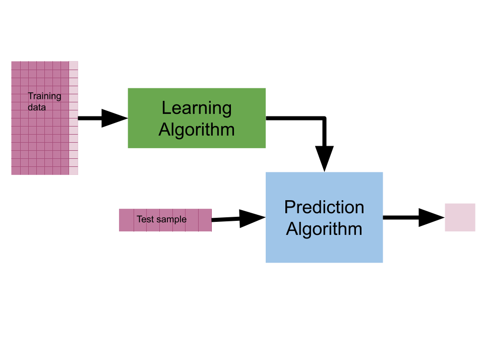
Figure 1:there are two types of algos
To do machine learning we start with training data which we put as input to the learning algorithm. A learning algorithm might be a generic optimization procedure or a specialized procedure for a specific model. The learning algorithm outputs a trained model or the parameters of the model. When we deploy a model we pair the fit model with a prediction algorithm or decision algorithm to evaluate a new sample in the world.
In experimenting and design, we need test data to evaluate how well our learning algorithm understood the world. We need to use previously unseen data, because if we don’t we can’t tell if the prediction algorithm is using a rule that the learning algorithm produced or just looking up from a lookup table the result. This can be thought of like the difference between memorization and understanding.
When the model does well on the training data, but not on test data, we say that it does not generalize well.