import pandas as pd
import numpy as np
import seaborn as sns

from sklearn.feature_extraction import text
from sklearn.metrics.pairwise import euclidean_distances
from sklearn import datasets
from scipy.special import expit
from sklearn.naive_bayes import MultinomialNB, GaussianNB
from sklearn import svm

from sklearn.neural_network import MLPClassifier
from sklearn.model_selection import train_test_split
from sklearn.metrics import confusion_matrix


sns.set_theme(palette='colorblind')
# edited so I can reuse these later
selected_categories = ['comp.graphics','sci.crypt']
ng_X,ng_y = datasets.fetch_20newsgroups(categories =selected_categories,
                                       return_X_y = True)
TF-IDF
This stands for term-frequency inverse document frequency. for a document number and word number with total documents:
where:
and
is the number of documents word occurs in
is te number of times word occurs in document
then sklearn also normalizes as follows:
tfidf = text.TfidfVectorizer()
ng_tfidf = tfidf.fit_transform(ng_X)ng_tfidf<Compressed Sparse Row sparse matrix of dtype 'float64'
with 188291 stored elements and shape (1179, 24257)>Now we can split the data.
ng_vec_train, ng_vec_test, ng_y_train, ng_y_test = train_test_split(ng_tfidf,ng_y)And we can fit a model:
clf_mnb = MultinomialNB()clf_mnb.fit(ng_vec_train,ng_y_train).score(ng_vec_test,ng_y_test)0.9593220338983051However, since this representation does not fit the asusmption of MutinomialNB (since it is no longer counts), this does worse than the one we fit on Tuesday with the CountVectorizer
This data is now normalized and continuous. An SVM is a better choice. We do not expect it to be linear, so we will set the rbf kernel, which allows it to make curved decision boundaries.
clf_tfidf = svm.SVC(kernel='rbf')and then fit and score:
clf_tfidf.fit(ng_vec_train,ng_y_train).score(ng_vec_test,ng_y_test)0.9830508474576272and this is even better than the MutinomialNB with the CountVectorizer representation
Distances in Text Data
Next we will take a few samples of each and see what the numerical representation gives us
Recall the two categories:
selected_categories['comp.graphics', 'sci.crypt']They’re in order so we can find the location of all the articles of each type:
first_graphics = np.where(ng_y == 0)[0]
first_crypt = np.where(ng_y == 1)[0]
where returns the indices where the condition is true in a tuple, so the last [0] just takes that set of indices out
and then pick those tow in a list:
subset_rows = np.concatenate([first_graphics,first_crypt])
subset_rows
array([ 0, 1, 3, ..., 1174, 1176, 1178], shape=(1179,))and finally we can compute the distances in the TF-IDF feature space from one article to another:
sns.heatmap( euclidean_distances(ng_tfidf[subset_rows]))<Axes: >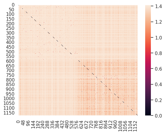
Sinve we have sorted the articles, the top left block is all graphics and the bottom right block is all cryptography. There are 0s (black) on the diagonal because every article’s distance to itself is 0.
This shows that the graphics articles are spread far apart from one another and distant from the cryptography ones (mostly lighter colors in the top left and the off digontal), but the cryptography articles are close together (the darker reds in the bottom right).
This mean thatt the cryptography articles are more similar to one another than they are to the graphics articles. It also shows that the cryptography articles are less diverse than the graphics articles.
We could also look at only the test samples, and we can sort them again too:
test_sorted = np.concatenate([np.where(ng_y_test == 0)[0],np.where(ng_y_test == 1)[0]])
sns.heatmap( euclidean_distances(ng_vec_test[test_sorted]))
<Axes: >
y_pred_tfidf = clf_tfidf.predict(ng_vec_test)
cols = pd.MultiIndex.from_arrays([['actual class']*len(selected_categories),
                                  selected_categories])
rows = pd.MultiIndex.from_arrays([['predicted class']*len(selected_categories),
                                  selected_categories])

pd.DataFrame(data = confusion_matrix(y_pred_tfidf,ng_y_test),columns = cols,
index = rows)This makes sense that more of the errors are mislabeling computer graphics as cryptography, since the graphics articles are more divers and the cryptography articles were mostly similar to one another.
What other models are there?
We have see a number of different classic machine learning models so far. The specific models we have seen so far all rely on a single common assumption: we can predict an outcome from inputs.
Review ML basics
Models in Machine Learning
Starting from a dataset, we first make an additional designation about how we will use the different variables (columns). We will call most of them the features, which we denote mathematically with and we’ll choose one to be the target or labels, denoted by .
The core assumption for just about all machine learning is that there exists some function so that for the th sample
would be the index of a DataFrame
is one value in the target column
is one row of the features
is a function that has parameters
We can then get different tasks given what we know when we train and a a machine learning algorithm, can be written like:
Most learning algorithms, assume a function class (e.g. linear or quadratic...)
The different types of ML are based on the availablity and type of outcome. Specific models relate to different assumptions about the form of the relationship.
In math:
what is determines the type of ML and the corresponds to different model or the different estimator objects (e.g. the MultinomialNB and SVC are different model classes).
We have found lots of models that work for lots of problems, but what if we do not have a good idea about what the function would look like?
Artificial Neurons
Early attempts at AI addressed this by drawing inspiration from biological neurons[1].
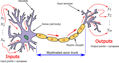
By Egm4313.s12 (Prof. Loc Vu-Quoc) - Own work, CC BY-SA 4.0, Link
Biological neurons have dendrites that synapse with other neurons and to sensory inputs (in the nose, eyes, skin, tongue, and ears) and interoceptive inputs (nerves throughout the body throug the spine and brainstem). As these inputs send chemical signals (called neurotransmitters) to the dendrtires through the synapse, the neurotransmitters allow ions to enter and change the charge of the cell’s body. If enough ions accumulate so that the charge exceeds a threshold a “spike” occurs: the cell body sends an electrical signal down that neuron’s axon to its terminals which release neurotransmitters to other synapses.
In the 1940s and 50s this was approximated by computer scientists:
for some nonlinear {term}`activation and they realized that by stacking (creating a network of them) these they could approximate a lot of different functions
That is we might have multiple hidden neurons that connects to our feature inputs () and then passes their output to another output neuron. So that with inputs( for ) and we can approximate , or compute
The original older name for these was a multilayer perceptron, so that is what sklearn calls it.
To rewrite in Python, an artificial neuron is a function that takes in 4 inputs and returns a value:
def aritificial_neuron_template(activation,weights,bias,inputs):
    '''
    simple artificial neuron

    Parameters
    ----------
    activation : function
      activation function of the neuron
    weights : numpy aray
      wights for summing inputs one per input
    bias: numpy array
      bias term added to the weighted sum
    inputs : numpy array
      input to the neuron, must be same size as weights

    '''
    return activation(np.matmul(inputs,weights) +bias)

#  common activation functions
identity_activation = lambda x: x
logistic_activation = lambda x: expit(x)
relu_activation = lambda x: np.max([np.zeros(x.shape),x],axis=0)
The logistic activation function squashes values to between 0 and 1:
x = np.linspace(-10,10)
sns.lineplot(x = x, y = logistic_activation(x))
<Axes: >
This is used for the output layer almost all the time.
The ReLU activation (rectified linear unit) makes negative numbers 0 and passes positive numbers through:
x = np.linspace(-10,10)
sns.lineplot(x = x, y = relu_activation(x))
<Axes: >
for a scalar input it would be the same as
relu_activation_scalar = lambda x: max(0,x)the extra stuff in the definition is to make it work with numpy arrays.
To find the values for the weights and the biases, we use numerical optimization of some sort. There are many ways to find the weights, but the basic idea is to optmize some objective function:
For binary classification we try to compute exactly the y as 0 or 1 and interpret the output as probability of . For more complex values we can use different activation functions for the output layer or for multiclass we 1 hot encode the classes and have multiple output neurons, one per class.
A simple MLP
Lets use a very simple dataset:
X, y = datasets.make_classification(n_samples=100, random_state=1,n_features=2,n_redundant=0)
X_train, X_test, y_train, y_test = train_test_split(X, y, stratify=y,
             random_state=1)
sns.scatterplot(x=X[:,0],y=X[:,1],hue=y)
<Axes: >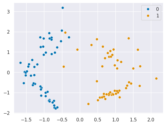
and fit an MLP to it
clf = MLPClassifier(
 hidden_layer_sizes=(1), # 1 hidden layer, 1 aritficial neuron
 max_iter=100, # maximum 100 interations in optimization
 alpha=1e-4, # regularization
 solver="lbfgs", #optimization algorithm
 verbose=10, # how much detail to print
 activation= 'identity' # how to transform the hidden layer beofore passing it to the next layer
)
clf.fit(X_train, y_train)

clf.score(X_test, y_test)1.0They are very good!
Now we will create a test point:
pt = np.array([-1,-2])and set up our network using our template function to verify how the predictions work:
hidden_neuron = lambda x: aritificial_neuron_template(identity_activation,clf.coefs_[0],
                                                      clf.intercepts_[0],x)
output_neuron = lambda h: aritificial_neuron_template(expit,clf.coefs_[1],
                                                    clf.intercepts_[1],h)

output_neuron(hidden_neuron(pt))array([0.00125393])the output of the hidden neuron fucntion hidden_neuron(pt) is the input to the outptut functionoutput_neuron.
We interpret this as the probability of it being in class 1:
this is the same as the predict_proba method:
clf.predict_proba([pt])array([[0.99874607, 0.00125393]])It holds for higher dimensions, too let’s make 4D data and fit an MLP to that:
X, y = datasets.make_classification(n_samples=200, random_state=1,n_features=4,n_redundant=0,n_informative=4)
X_train, X_test, y_train, y_test = train_test_split(X, y, stratify=y,
                          random_state=5)
pt_4d =np.asarray([[-1,-2,2,-1],[1.5,0,.5,1]])
clf_4d = MLPClassifier(
  hidden_layer_sizes=(1),
  max_iter=5000,
  alpha=1e-4,
  solver="lbfgs",
  verbose=10,
  activation= 'identity'
)

clf_4d.fit(X_train, y_train)
clf_4d.score(X_test, y_test)0.84Not as good, but still not bad, with only one hidden neuron. We can again create the neural network:
This time has 2 points, so we have 2 probabilities.
and again this probability of predicting 1 matches:
clf_4d.predict_proba(pt_4d)array([[0.04642966, 0.95357034],
[0.14667997, 0.85332003]])the first element is probability of 0 and the second probability of 1.
We can also total up how many parameters there are by looking at them
clf_4d.coefs_[0],clf_4d.coefs_[1], clf_4d.intercepts_[0], clf_4d.intercepts_[1](array([[ 0.42071889],
[-1.95894733],
[-0.5333183 ],
[ 0.37329427]]),
array([[0.95594028]]),
array([0.50923262]),
array([0.56887558]))While we can map what these parameters are used for in the equations, these parameters are not interpretable. They do not tell us anything about our features or the relationship. ANNs are very effective, but not interpretable by default.
Or only sum them up:
n_param = np.prod(clf_4d.coefs_[0].shape) + np.prod(clf_4d.coefs_[1].shape) + len(clf_4d.intercepts_[0]) + len(clf_4d.intercepts_[1])
n_paramnp.int64(7)This is a small number, recall that LLMs are hundreds of billions of parameters.
Two hidden neurons
Let’s try to improve that model. We will use 4 hidden neurons and the ReLU activation function:
clf_4d_2 = MLPClassifier(
  hidden_layer_sizes=(4),
  max_iter=5000,
  alpha=1e-4,
  solver="lbfgs",
  verbose=10,
  activation= 'relu'
)

clf_4d_2.fit(X_train, y_train)
clf_4d_2.score(X_test, y_test)0.98That is a better performance than before!
Now it has more parameters too:
sum([np.prod(c.shape) for c in clf_4d_2.coefs_]) + sum([len(i) for i in clf_4d.intercepts_])np.int64(22)We can implement this with out simple tempalte to verify how it works for the predictions:
hidden_neuron_4d_0 = lambda x: aritificial_neuron_template(relu_activation,
                             clf_4d_2.coefs_[0][:,0],clf_4d_2.intercepts_[0][0],x)
hidden_neuron_4d_1 = lambda x: aritificial_neuron_template(relu_activation,
                             clf_4d_2.coefs_[0][:,1],clf_4d_2.intercepts_[0][1],x)
hidden_neuron_4d_2 = lambda x: aritificial_neuron_template(relu_activation,
                             clf_4d_2.coefs_[0][:,2],clf_4d_2.intercepts_[0][2],x)
hidden_neuron_4d_3 = lambda x: aritificial_neuron_template(relu_activation,
                             clf_4d_2.coefs_[0][:,3],clf_4d_2.intercepts_[0][3],x)
output_neuron_4d_2 = lambda x: aritificial_neuron_template(logistic_activation,
                             clf_4d_2.coefs_[1],clf_4d_2.intercepts_[1],x)


output_neuron_4d_2(np.asarray([hidden_neuron_4d_0(pt_4d),
                              hidden_neuron_4d_1(pt_4d),
                              hidden_neuron_4d_2(pt_4d),
                              hidden_neuron_4d_3(pt_4d)]).T)
array([[9.99999516e-01],
[1.05122633e-07]])Again the one output neuron gets the 4 hidden neurons as its input. Tthey need to be transposed after stacking to put them back to being the rows. and these are the probabilities of 1 for our two samples:
clf_4d_2.predict_proba(pt_4d)array([[4.84065329e-07, 9.99999516e-01],
[9.99999895e-01, 1.05122633e-07]])Notice that it make sthe same predictions for the test samples, but this model is more confident (the numbers are more extreme) than the smaller model
Questions
this is based on an understanding of isolated neurons and a coarse approximation, biological neural networks (aka. brains) are a lot more complex than any ANN architecture. At minimum, because they are modulated by many chemicals and there are other cells besides neurons that are important.