Model Optimization

import matplotlib.pyplot as plt
import numpy as np
import seaborn as sns
import pandas as pd
from sklearn import datasets
from sklearn import cluster
from sklearn import svm, datasets
from sklearn.model_selection import GridSearchCV
from sklearn.model_selection import train_test_split
from sklearn import tree

Train, test and Validation data¶

We will work with the iris data again.

iris_df = sns.load_dataset('iris')

iris_X = iris_df.drop(columns=['species'])

iris_y = iris_df['species']

We will still use the test train split to keep our test data separate from the data that we use to find our preferred parameters.

iris_X_train, iris_X_test, iris_y_train, iris_y_test = train_test_split(iris_X,iris_y, random_state=0)

We will be doing cross validation late, but we still use train_test_split at the start that we have the true test data

Think Ahead¶

• What would you need to be able to find the best parameter settings?

• what would be the inputs to an algorithm to optimize a model

• what might the steps include?

Setting up model optmization¶

Today we will optimize a decision tree over three parameters.

One is the criterion, which is how it decides where to create thresholds in parameters. Gini is the default and it computes how concentrated each class is at that node, another is entropy, which is a measure of how random something is. Intuitively these do similar things, which makes sense because they are two ways to make the same choice, but they have slightly different calculations.

The other two parameters relate to the structure of the decision tree that is produced and their values are numbers.

• max_depth is the height of the tree

• min_samples_leaf per leaf makes it keeps the leaf sizes small.

dt = tree.DecisionTreeClassifier()
params_dt = {'criterion':['gini','entropy'],
             'max_depth':[2,3,4],
       'min_samples_leaf':list(range(2,20,2))}

Grid Search¶

We will first to an exhaustive optimization on that parameter grid, params_dt.

The dictionary is called a parameter grid because it will be used to create a “grid” of different values, by taking every possible combination.

The GridSearchCV object will then also do cross validation, with the same default values we saw for cross_val_score of 5 fold cross validation (Kfold with K=5).

num_param_values = {k:len(v) for k,v in params_dt.items()}
num_param_values

combos = np.prod([v for v in num_param_values.values()])
combos

We will instantiate it it with default CV settings.

dt_opt = GridSearchCV(dt,params_dt)

The GridSearchCV keeps the same basic interface of estimator objects, we run it with the fit method.

dt_opt.fit(iris_X_train,iris_y_train)

We can also get predictions, from the model with the highest score out of all of the combinations:

y_pred = dt_opt.predict(iris_X_test)

we can also score it as normal.

test_score = dt_opt.score(iris_X_test,iris_y_test)
test_score

This is our true test accuracy because this data iris_X_test,iris_y_test was not used at all for training or for optimizing the parameters.

we can also see the best parameters.

dt_opt.best_params_

Grid Search Results¶

The optimizer saves a lot of details of its process in a dictionary

dt_opt.cv_results_

It is easier to work with if we use a DataFrame:

dt_5cv_df = pd.DataFrame(dt_opt.cv_results_)

First let’s inspect its shape:

dt_5cv_df.shape

Notice that it has one row for each of the np.int64(54) combinations we computed above).

It has a lot of columns, we can use the head to see them

dt_5cv_df.head()

• the fit_time is the time it takes for the .fit method to run for a single setting of hyperparameter values. it computes the mean and std of these over the Kfold cross validation (so here, over 5 separate times)

• the score_time is the time to make predictions. it computes the mean and std of these over the Kfold cross validation (so here, over 5 separate times)

• there is one param_ column for each key in the parameter grid (<function dict.keys>)

• the params column contains a dictionary of all of the parameters used for that row

• the test_scores are better termed the validation accuracy because is truly the score for the validation data it is the “test” set from the splits in the cross validation loop. It records the value for each fold, the mean and the std for them.

• rank_test_score is the rank for that hyperparameter setting’s mean_test_score

Since we used a classifier here, the score is accuracy if it was regression it would be the $R^2$ score, if Kmeans it would be the opposite of the Kmeans objective.

We can also plot the dta and look at the performance.

sns.catplot(data=dt_5cv_df,x='param_min_samples_leaf',y='mean_test_score',
           col='param_criterion', row= 'param_max_depth', kind='bar',)

<seaborn.axisgrid.FacetGrid at 0x7f194a4f8ec0>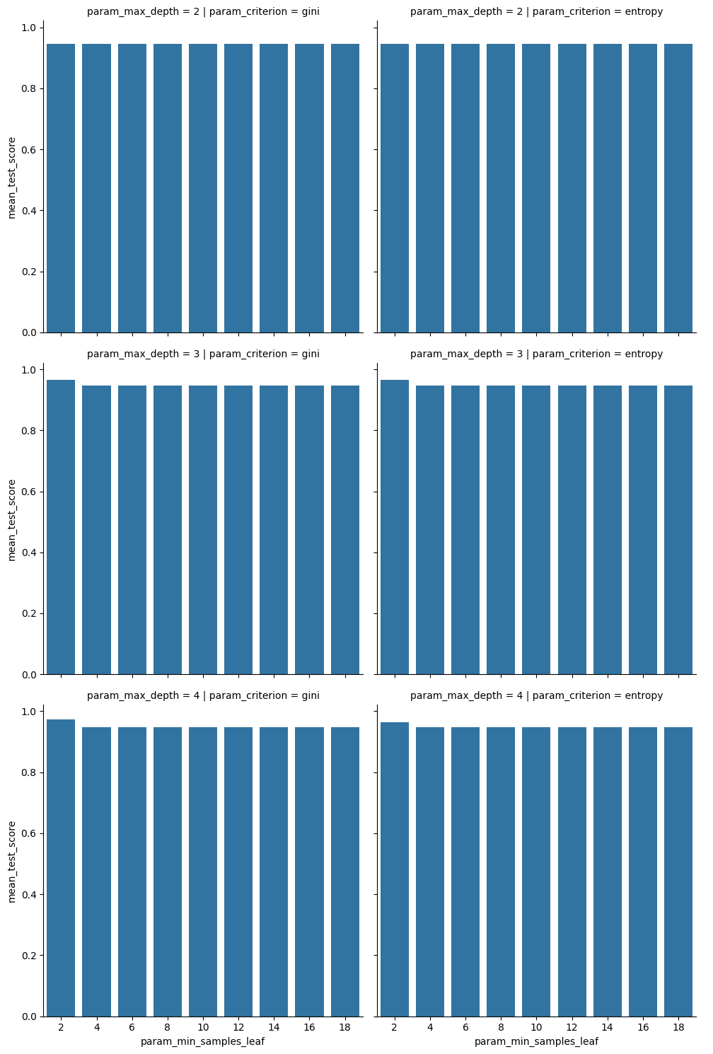

this makes it clear that none of these stick out much in terms of performance.

The best model here is not much better than the others, but for less simple tasks there are more things to choose from.

Impact of CV parameters¶

Let’s fit again with cv=10 to see with 10-fold cross validation.

dt_opt10 = GridSearchCV(dt,params_dt,cv=10)
dt_opt10.fit(iris_X_train,iris_y_train)

and get the dataframe for the results

dt_10cv_df = pd.DataFrame(dt_opt10.cv_results_)

We can stack the columns we want from the two results together with a new indicator column cv:

plot_cols = ['param_min_samples_leaf','std_test_score','mean_test_score',
             'param_criterion','param_max_depth','cv']
dt_10cv_df['cv'] = 10
dt_5cv_df['cv'] = 5

dt_cv_df = pd.concat([dt_5cv_df[plot_cols],dt_10cv_df[plot_cols]])
dt_cv_df.head()

this can be used to plot.

sns.catplot(data=dt_cv_df,x='param_min_samples_leaf',y='mean_test_score',
           col='param_criterion', row= 'param_max_depth', kind='bar',
           hue = 'cv')

<seaborn.axisgrid.FacetGrid at 0x7f1948924530>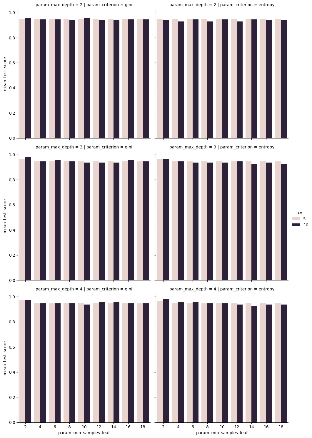

we see that the mean scores are not very different, but that 10 is a little higher in some cases. This makes sense, it has more data to learn from, so it found something that applied better, on average, to the test set.

sns.catplot(data=dt_cv_df,x='param_min_samples_leaf',y='std_test_score',
           col='param_criterion', row= 'param_max_depth', kind='bar',
           hue = 'cv')

<seaborn.axisgrid.FacetGrid at 0x7f194895ec90>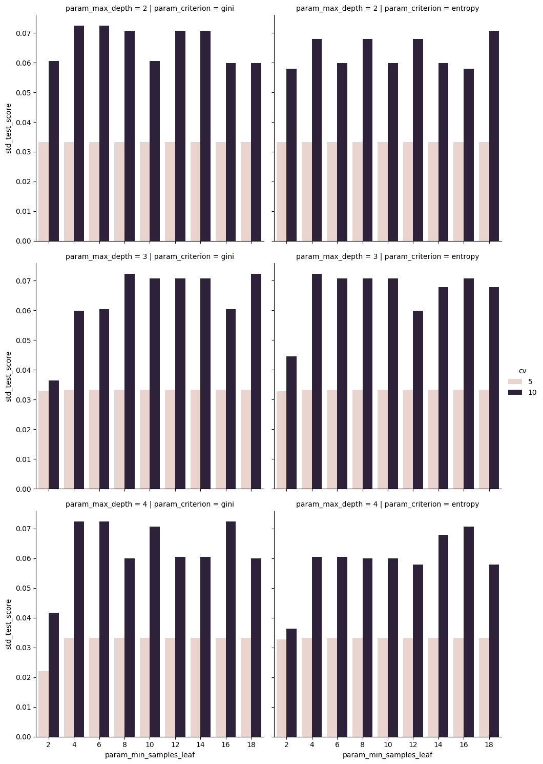

However here we see that the variabilty in those scores is much higher, so maybe the 5 is better.

There were a really small number of samples used to compute each of those scores so some of them will vary a lot more.

.75*150

112/5

We can compare to see if it finds the same model as best:

dt_opt.best_params_

dt_opt10.best_params_

In some cases they will and others they will not.

dt_opt.score(iris_X_test,iris_y_test)

dt_opt10.score(iris_X_test,iris_y_test)

In some cases they will find the same model and score the same, but it other time they will not.

The takeaway is that the cross validation parameters impact our ability to measure the score and possibly how close that cross validation mean score will match the true test score. Mostly it will change the variability in the estimate of the score. It does not change necessarily which model is best, that is up to the data iteself (the original test/train split would impact this).

Other searches¶

from sklearn import model_selection
from sklearn.model_selection import LeaveOneOut

rand_opt = model_selection.RandomizedSearchCV(dt,params_dt,)
rand_opt.fit(iris_X_train, iris_y_train)

rand_opt.score(iris_X_test,iris_y_test)

It might find the same solution, but it also might not. If you do some and see that the parameters overall do not impact the scores much, then you can trust whichever one, or consider other criteria to choose the best model to use.

Choosing a model to use¶

The Grid search finds the hyperparameter values that result in the best mean score. But what if more than one does that?

dt_5cv_df['rank_test_score'].value_counts()

Lets look at the ones sharing a rank of 1:

dt_5cv_df[dt_5cv_df['rank_test_score']==1]

We can compare on other aspects, like the time. In particular a lower or more consistent score_time could impact how expensive it is to run your model in production.

dt_5cv_df[['mean_fit_time', 'std_fit_time', 'mean_score_time', 'std_score_time']].mean()

dt_5cv_df[['mean_fit_time', 'std_fit_time', 'mean_score_time', 'std_score_time']].head(3)

Questions After Class¶