Task Review and Cross Validation

This week we will learn to optimize models, or find the best hyperparameters for the models that make them fit data best. Next week will study another topic in model selection: model comparison. First, we will review the task types so that we can be sure that we are applying models in the right contexts.

In order to optimize the parameters, then we need to be able to compare the model’s performance with one set of hyperparameter values to another. To do this, we need to be sure we have a very good, reliable, measure of how good the model is.

Note have seen that the test train splits, which are random, influence the performance.

In order to find the best hyperparameters for the model on a given dataset, we need some better evaluation techniques. Today we will study how to do this.

ML Tasks¶

We learned classification first, because it shares similarities with each regression and clustering, while regression and clustering have less in common.

• Classification is supervised learning for a categorical target.

• Regression is supervised learning for a continuous target.

• Clustering is unsupervised learning for a categorical target.

We have used a small flowchart for the tasks:

Sklearn provides a nice flow chart for thinking through both tasks (big blocks) and models (the small green boxes)

Predicting a category is another way of saying categorical target. Predicting a quantitiy is another way of saying continuous target. Having labels or not is the difference between supervised and unsupervized learning.

The flowchart assumes you know what you want to do with data and that is the ideal scenario. You have a dataset and you have a goal. For the purpose of getting to practice with a variety of things, in this course we ask you to start with a task and then find a dataset. Assignment 9 is the last time that’s true however. Starting with Assignment 10, you can choose and focus on a specific application domain and then choose the right task from there.

Thinking about this, however, you use this information to move between the tasks within a given type of data. For example, you can use the same data for clustering as you did for classification. Switching the task changes the questions though:

• classification evaluation tells us how separable the classes are given that classifiers decision rule

• Clustering can find other subgroups or the same ones, so the evaluation we choose allows us to explore this in more ways.

Regression requires a continuous target, so we need a dataset to be suitable for that; we can’t transform from the classification dataset to a regression one.
However, we can go the other way and that’s how some classification datasets are created.

For example, the very popular, UCI adult Dataset is a popular ML dataset that was dervied from census data. The goal is to use a variety of features to predict if a person makes more than $50k per year or not. While income is a continuous value, they applied a threshold ($50k) to it to make a binary variable. The dataset does not include income in dollars, only the binary indicator.

Recent work reconstructed the dataset with the continuous valued income. Their repository contains the data as well as links to their paper and a video of their talk on it.

# basic libraries
import numpy as np
import pandas as pd
import seaborn as sns
import matplotlib.pyplot as plt
# models classes
from sklearn import tree
from sklearn import cluster
from sklearn import svm
# datasets
from sklearn import datasets
# model selection tools
from sklearn.model_selection import GridSearchCV
from sklearn.model_selection import cross_val_score
from sklearn.model_selection import train_test_split
from sklearn.model_selection import KFold, ShuffleSplit
from sklearn import metrics

Why Better Evaluation?¶

Before we do better evaluation on our actual models, let’s build some intuition for a random experiment overall.

Let’s consider a simple experiment to detect if a coin is fair or not.

We’ll define a little tiny object

class Coin:
    def __init__(self,p):
        '''
        set Probability of 'heads'
        '''
        self.p = {'heads':p,'tails':1-p}

    def flip(self):
        return str(np.random.choice(list(self.p.keys()),
                        p=list(self.p.values())))
    
    def get_p(side):
        return self.p[side]

and we’ll set up two coins:

fair_coin = Coin(.5)
biased_coin = Coin(.75)

We can now flip the fair coin, and say we get heads and we can get the biased coin as well and we get heads. From one flip of either coin, we cannot tell the difference in either of them, but if we flip more times we can look at the pattern.

If we flip each 10 times and then sort the answers, we can count the heads and divide by 10 to get the estimate of the coin’s probability of heads (which are set to {'heads': 0.5, 'tails': 0.5} and {eval})

N = 10
fair_flips10_1 = sorted([fair_coin.flip() for i in range(N)])
bias_flips10_1  = sorted([biased_coin.flip() for i in range(N)])
fair_flips10_1.count('heads')/N, bias_flips10_1.count('heads')/N

But if we repeat that, we will probably get a different result

fair_flips10_2  = sorted([fair_coin.flip() for i in range(N)])
bias_flips10_2  = sorted([biased_coin.flip() for i in range(N)])
fair_flips10_2 .count('heads')/N, bias_flips10_2.count('heads')/N

If instead we flip each 100 times,

N = 100
fair_flips100_1  = sorted([fair_coin.flip() for i in range(N)])
bias_flips100_1 = sorted([biased_coin.flip() for i in range(N)])
fair_flips100_1.count('heads')/N, bias_flips100_1.count('heads')/N

and do that a second time

fair_flips100_2 = sorted([fair_coin.flip() for i in range(N)])
bias_flips100_2 = sorted([biased_coin.flip() for i in range(N)])
fair_flips100_2.count('heads')/N, bias_flips100_2.count('heads')/N

the difference between the two trials of 100 (0.5 vs 0.46 and 0.75 vs 0.73) is probably smaller than the ones for 10 (0.2 vs 0.6and 0.5 vs 0.7)

So if we formalize this our estimate of the $P(heads)$ based on different numbers of N:

N_list = [5,10,25,50,100,250, 500, 750, 1000]
dat = []
for rep in range(10):
    for N in N_list: 
        fair_est_p = sorted([fair_coin.flip() for i in range(N)]).count('heads')/N
        bias_est_p = sorted([biased_coin.flip() for i in range(N)]).count('heads')/N
        dat.append([rep, N, fair_est_p, bias_est_p])

df = pd.DataFrame(dat, columns= ['repetition','N','fair','bias']).melt(id_vars=['repetition','N'],value_vars = ['fair','bias'],value_name='est_p',var_name = 'coin')
df.head()

log N

Linear N

g = sns.relplot(df, x='N',y='est_p',hue='coin',col='coin')
g.set(xscale="log")

<seaborn.axisgrid.FacetGrid at 0x7f365eac1820>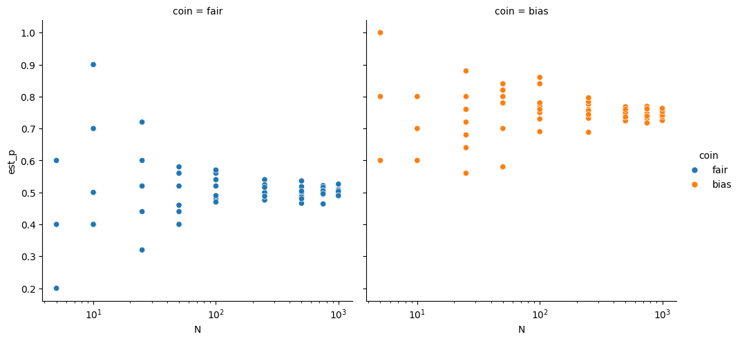

g = sns.relplot(df, x='N',y='est_p',hue='coin',col='coin')
g.set(xscale="linear")

<seaborn.axisgrid.FacetGrid at 0x7f365e7e9ac0>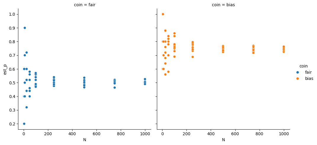

For small values of N, the two coins are hard to differentiate, we might not be able to tell the difference betweent the two. With larger N, however, we can separate the two very well.

This is like with our models, if we have a small number of test samples, or an unreliable test score, we might get nearly the same values for different hyperparameter values that actually would.

K-fold Cross Validation¶

This way we can get dataFrames:

iris_X, iris_y = datasets.load_iris(return_X_y=True,as_frame=True)

and instantiate a Decision tree

dt = tree.DecisionTreeClassifier()

We can split the data, fit the model, then compute a score, but since the splitting is a randomized step, the score is a random variable.

For example, if we have a coin that we want to see if it’s fair or not. We would flip it to test. One flip doesn’t tell us, but if we flip it a few times, we can estimate the probability it is heads by counting how many of the flips are heads and dividing by how many flips.

We can do something similar with our model performance. We can split the data a bunch of times and compute the score each time.

cross_val_score does this all for us.

It takes an estimator object and the data.

By default it uses 5-fold cross validation. It splits the data into 5 sections, then uses 4 of them to train and one to test. It then iterates through so that each section gets used for testing.

cross_val_score(dt,iris_X, iris_y)

We get back a score for each section or “fold” of the data. We can average those to get a single estimate.

To actually report, we would take the mean

np.mean(cross_val_score(dt,iris_X, iris_y))

We can change from 5-fold to 10-fold by setting the cv parameter

cross_val_score(dt,iris_X, iris_y,cv=10)

In K-fold cross validation, we split the data in K sections and train on K-1 and test one 1 section. So the percentages are like:

# K is the cv
K = 10
train_pct =(K-1)/K
test_pct = 1/K
train_pct, test_pct

and we can re calculate for a different K

# K is the / numbr of folds
K = 7
train_pct = (K-1)/K
test_pct = 1/K
train_pct, test_pct

Cross validation is model-agnostic¶

We can use any estimator object here.

For example, we can apply it to clustering too:

km = cluster.KMeans(n_clusters = 3)

cross_val_score(km, iris_X)

To see what this score is, we can look at the help

help(km.score)

Help on method score in module sklearn.cluster._kmeans:

score(X, y=None, sample_weight=None) method of sklearn.cluster._kmeans.KMeans instance
    Opposite of the value of X on the K-means objective.

    Parameters
    ----------
    X : {array-like, sparse matrix} of shape (n_samples, n_features)
        New data.

    y : Ignored
        Not used, present here for API consistency by convention.

    sample_weight : array-like of shape (n_samples,), default=None
        The weights for each observation in X. If None, all observations
        are assigned equal weight.

    Returns
    -------
    score : float
        Opposite of the value of X on the K-means objective.

KFold Details¶

First, lets look at the Kfold cross validation object. Under the hood, this is the default thing that cross_val_score uses ^[1]

Cross validation objects are all examples of the splitter type in sklearn

we can instantiate one of these too:

kf = KFold(n_splits=10)

it returns the splits as a generator

type(range(3))

range(3)

list(range(3))

[i for i in range(3)]

splits = kf.split(iris_X,iris_y)
splits

jupyter does not know how to display it, so it jsut says the type.

type(splits)

We can use this in a loop to get the list of indices that will be used to get the test and train data for each fold. To visualize what this is doing, see below.

N_samples = len(iris_y)
def gen_kf_tt_df(splitter):
    kf_tt_list = []
    i = 1
    for train_idx, test_idx in splitter:
        
        # make a list of "3"
        col_data =  np.asarray([3]*N_samples)
        # fill in train and test by the indices
        col_data[train_idx] = 0
        col_data[test_idx] = 1
        kf_tt_list.append(pd.DataFrame(data = col_data,index=list(range(N_samples)), columns = ['split ' + str(i)]))
        i +=1

    df = pd.concat(kf_tt_list,axis=1)
    return df

This small experiment iterates over the split obect and then puts 0 for ‘Train’ or 1 for ‘Test’ in the elements of an array in the locations selected for each role. We convert that array to a DataFrame with a column title and stack them together.

when we run it:

kf_tt_df = gen_kf_tt_df(splits)
kf_tt_df.head()

We end up with a DataFrame with columns for each split (Index(['split 1', 'split 2', 'split 3', 'split 4', 'split 5', 'split 6', 'split 7', 'split 8', 'split 9', 'split 10'], dtype='object')) with the labels of 0 for train or 1 for test.

This dataframe is most useful for visualizing what it means to split the data into K folds:

cmap = sns.color_palette("tab10",10)
g = sns.heatmap(kf_tt_df,cmap=cmap[7:9],cbar_kws={'ticks':[.25,.75]},linewidths=0,
    linecolor='gray')
colorbar = g.collections[0].colorbar
colorbar.set_ticklabels(['Train','Test'])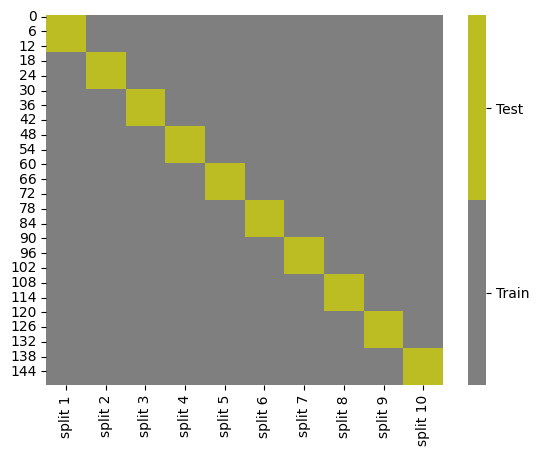

or we can do other values of K

K= 5

K= 7

K= 25

K= 50

K= 150

splits = KFold(n_splits=5).split(iris_X,iris_y)
kf_tt_df = gen_kf_tt_df(splits)
kf_tt_df.head()
cmap = sns.color_palette("tab10",10)
g = sns.heatmap(kf_tt_df,cmap=cmap[7:9],cbar_kws={'ticks':[.25,.75]},linewidths=0,
    linecolor='gray')
colorbar = g.collections[0].colorbar
colorbar.set_ticklabels(['Train','Test'])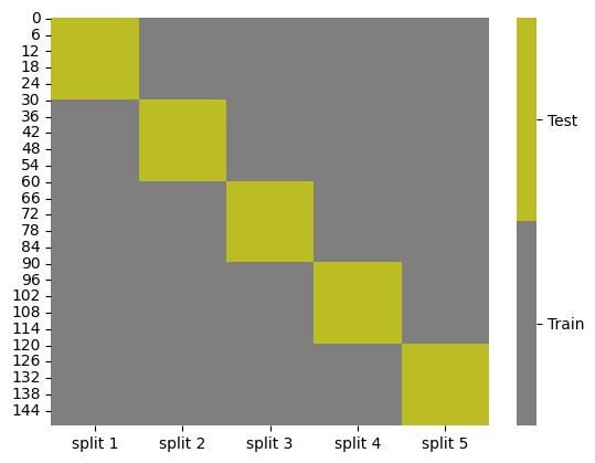

splits = KFold(n_splits=7).split(iris_X,iris_y)
kf_tt_df = gen_kf_tt_df(splits)
kf_tt_df.head()
cmap = sns.color_palette("tab10",10)
g = sns.heatmap(kf_tt_df,cmap=cmap[7:9],cbar_kws={'ticks':[.25,.75]},linewidths=0,
    linecolor='gray')
colorbar = g.collections[0].colorbar
colorbar.set_ticklabels(['Train','Test'])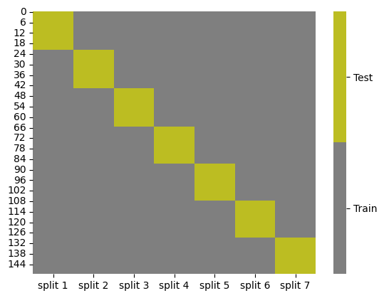

splits = KFold(n_splits=25).split(iris_X,iris_y)
kf_tt_df = gen_kf_tt_df(splits)
kf_tt_df.head()
cmap = sns.color_palette("tab10",10)
g = sns.heatmap(kf_tt_df,cmap=cmap[7:9],cbar_kws={'ticks':[.25,.75]},linewidths=0,
    linecolor='gray')
colorbar = g.collections[0].colorbar
colorbar.set_ticklabels(['Train','Test'])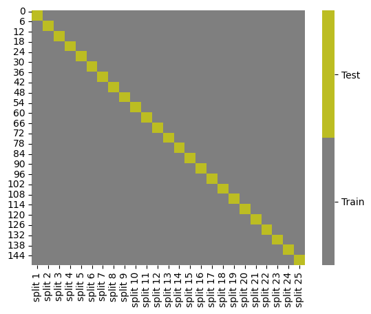

splits = KFold(n_splits=50).split(iris_X,iris_y)
kf_tt_df = gen_kf_tt_df(splits)
kf_tt_df.head()
cmap = sns.color_palette("tab10",10)
g = sns.heatmap(kf_tt_df,cmap=cmap[7:9],cbar_kws={'ticks':[.25,.75]},linewidths=0,
    linecolor='gray')
colorbar = g.collections[0].colorbar
colorbar.set_ticklabels(['Train','Test'])

splits = KFold(n_splits=150).split(iris_X,iris_y)
kf_tt_df = gen_kf_tt_df(splits)
kf_tt_df.head()
cmap = sns.color_palette("tab10",10)
g = sns.heatmap(kf_tt_df,cmap=cmap[7:9],cbar_kws={'ticks':[.25,.75]},linewidths=0,
    linecolor='gray')
colorbar = g.collections[0].colorbar
colorbar.set_ticklabels(['Train','Test'])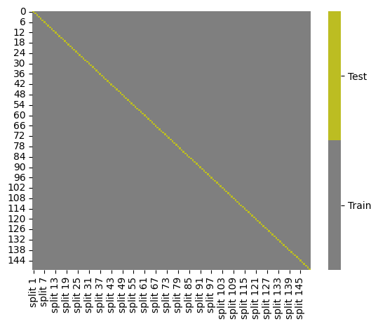

The last case above K=150, is also K=N, that the number of folds is equal to the number of samples. That is why this is also called leave one out cross validation because there is one sample used to test in each case, or one sample left out from training each time.

Note that unlike test_train_split this does not always randomize and shuffle the data before splitting.

ShuffleSplit Cross Validation¶

We can also see another splitter(this is what train_test_split uses)

skf = ShuffleSplit(10)

splits = skf.split(iris_X,iris_y)
skf_tt_df = gen_kf_tt_df(splits)
skf_tt_df.head()
cmap = sns.color_palette("tab10",10)
g = sns.heatmap(skf_tt_df,cmap=cmap[7:9],cbar_kws={'ticks':[.25,.75]},linewidths=0,
    linecolor='gray')
colorbar = g.collections[0].colorbar
colorbar.set_ticklabels(['Train','Test'])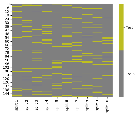

we can see this is different and more random.

We can also use it in cross_val_score and with any number of splits we want:

cross_val_score(dt,iris_X,iris_y,cv=ShuffleSplit(n_splits=100,test_size=.2))

We all ran this code and got very similar numbers:

np.mean(cross_val_score(dt,iris_X,iris_y,cv=ShuffleSplit(n_splits=100,test_size=.2)))

and this one and got widely varying numbers:

iris_X_train, iris_X_test, iris_y_train, iris_y_test = train_test_split(iris_X,iris_y,test_size=.2)
dt.fit(iris_X_train,iris_y_train).score(iris_X_test, iris_y_test)

To emulate that experiment we did as a group in class, I’ll repeat both with loops here:

n_reps = 30
shuffle100mean = [np.mean(cross_val_score(dt,iris_X,iris_y,cv=ShuffleSplit(n_splits=100,test_size=.2))) for i in range (n_reps)]

def split_train():
    iris_X_train, iris_X_test, iris_y_train, iris_y_test = train_test_split(iris_X,iris_y,test_size=.2)
    return dt.fit(iris_X_train,iris_y_train).score(iris_X_test, iris_y_test)

single_score = [split_train() for i in range (n_reps)]

Then we can look at the values 30 reps of the mean of 100 Shufflesplits: [np.float64(0.943666666666667), np.float64(0.9476666666666667), np.float64(0.9460000000000001), np.float64(0.9473333333333335), np.float64(0.9516666666666669), np.float64(0.9486666666666669), np.float64(0.9476666666666668), np.float64(0.949666666666667), np.float64(0.9500000000000003), np.float64(0.9460000000000001), np.float64(0.9456666666666669), np.float64(0.9520000000000002), np.float64(0.9480000000000003), np.float64(0.9506666666666669), np.float64(0.943), np.float64(0.9456666666666669), np.float64(0.9513333333333336), np.float64(0.9456666666666669), np.float64(0.9383333333333335), np.float64(0.9483333333333335), np.float64(0.9433333333333336), np.float64(0.9530000000000001), np.float64(0.9423333333333335), np.float64(0.9473333333333338), np.float64(0.9416666666666669), np.float64(0.9423333333333334), np.float64(0.9470000000000002), np.float64(0.9483333333333335), np.float64(0.9453333333333336), np.float64(0.9466666666666669)]

or 30 reps of a single split, train, and score: [0.9666666666666667, 0.9333333333333333, 1.0, 0.9333333333333333, 0.9666666666666667, 0.9, 0.9, 0.9, 0.8333333333333334, 1.0, 0.9333333333333333, 0.9666666666666667, 0.9, 0.9666666666666667, 0.9333333333333333, 0.9666666666666667, 0.9, 1.0, 0.9333333333333333, 0.9, 0.9666666666666667, 0.8333333333333334, 0.9666666666666667, 1.0, 1.0, 0.9666666666666667, 0.9, 1.0, 0.9666666666666667, 0.9666666666666667]

We not see how spread out these values are:

np.std(shuffle100mean)

np.std(single_score)

The values are much more consistent for the Shufflesplit. If a data scientist evaluates their model only once, with a single train test split, you could get lucky or unlucky and get a high (e.g. np.float64(1.0)) or low(e.g. np.float64(0.8333333333333334)) value. But with the 100 trials averaged together it is more consisten with the difference between the max and min much smaller: np.float64(0.01) (np.float64(0.9530000000000001) vs np.float64(0.9383333333333335))

We can do this again for a single trial, saving the results:

score_list = cross_val_score(dt,iris_X,iris_y,cv=ShuffleSplit(n_splits=100,test_size=.2))

We get a good mean and a small std:

np.mean(score_list), np.std(score_list)

but with fewer trials the std is larger

np.std(cross_val_score(dt,iris_X,iris_y,cv=ShuffleSplit(n_splits=10,test_size=.2)))

Questions¶

In last class’s notes, you gave us the option to submit a question as an issue on the repo for extra credit. Would this be under the “Question” issue, or is that issue only for assignment questions?¶

That is for anything general about content in this material (notes, assignments, resources). It should not include questions that show your work on an assignment (put those in your portfolio repo)

Can we submit questions for older class notes as well if we have them?¶

yes!

how do I choose the right K?¶

To choose the right K for K fold, you have to balance how complex the problem is, how much data you have and how reliable you need your test score to be. Those will have different importances in different contexts.

If you have a complex problem, you need more data for training (remember the diabetes model performed bettter with 95% training data (20 samples test) than with 75% training data).

If you do not have a lot of data you may want to train on as much as possible to leave one out cross validation (K=N for N samples) might be good.

If you need to really trust the test score, you need to have enough data in testing, but any cross validation allows you to get more test data, so you can use any to improve this. A shuffle split where samples are used more than once might be good for this.

when we use the cross_val_score and get an array, what do all of those numbers mean?¶

For classifiers, they are the accuracy of all the different trials. For regression it is the $R^2$ score. For Kmeans it is the Kmeans default score of the opposite of the kmeans objective function.