Today we are going to see a second classification model.
Last class we saw Gaussian Naive Bayes. The model class, or model determines what assumptions we are making before we fit the model to the data. The model specifies the mathematical form of the prediction algorithm and determines what the learning algorithm must do. For many model there exist multiple valid learning algorithms, and some learning algorithms can learn the parameters of multiple model classes, because the learning algorithm is often an optimization algorithm of some sort.
import pandas as pd
import seaborn as sns
import numpy as np
from sklearn import tree
import matplotlib.pyplot as plt
from sklearn.model_selection import train_test_split
from sklearn.naive_bayes import GaussianNB
from sklearn import metrics
sns.set(palette='colorblind') # this improves contrast

from sklearn.metrics import confusion_matrix, classification_report

from IPython.display import display
corner_data = 'https://raw.githubusercontent.com/rhodyprog4ds/06-naive-bayes/f425ba121cc0c4dd8bcaa7ebb2ff0b40b0b03bff/data/dataset6.csv'
df6= pd.read_csv(corner_data,usecols=[1,2,3])What if the assumptions are not met?
Using a toy dataset here shows an easy to see challenge for the classifier that we have seen so far. Real datasets will be hard in different ways, and since they’re higher dimensional, it’s harder to visualize the cause.
First let’s take a look at the structre of the dataset:
df6.head()It is very simple, it has two continuous features x0 and x1 and one categorical variable, char that we will use as a target variable.
We can look at a pairplot to get a better picture:
sns.pairplot(data=df6, hue='char', hue_order=['A','B'])<seaborn.axisgrid.PairGrid at 0x7efe2a7a7800>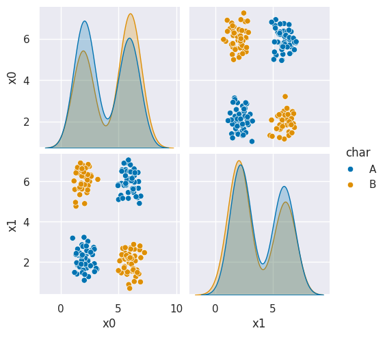
As we can see in this dataset, these classes are quite separated.
To do any ML we have to split the data into train and test sets. We will also set a random state.
random_state0 = 67
X_train, X_test, y_train, y_test = train_test_split(df6[['x0','x1']],df6['char'],
                                                    random_state =random_state0)
We will next instantiate a GNB object:
gnb = GaussianNB()and fit and score:
gnb.fit(X_train, y_train)
gnb.score(X_test,y_test)0.56This is not a very good score, even though the data looked very separable.
To see why, we can look at what it learned.
We will again sample from the generative model
N = 100
gnb_df = pd.DataFrame(np.concatenate([np.random.multivariate_normal(th, sig*np.eye(2),N)
         for th, sig in zip(gnb.theta_,gnb.var_)]),
         columns = ['x0','x1'])
gnb_df['char'] = [ci for cl in [[c]*N for c in gnb.classes_] for ci in cl]

sns.pairplot(data =gnb_df, hue='char',hue_order=['A','B'])
<seaborn.axisgrid.PairGrid at 0x7efe2a458cb0>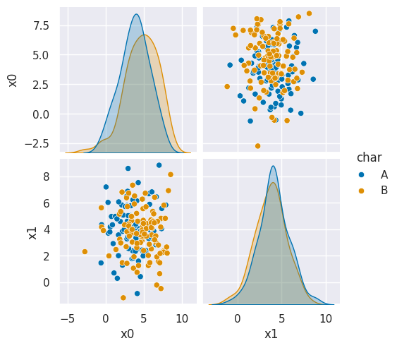
In this example, we can see it learned nearly the same mean and variance for both classes so it learned the classes as basically completely overlapping.
We can also inspect the means: array([[3.85630137, 3.92739726], [4.41298701, 3.64454545]]) and variances: array([[3.74042057, 3.83637816], [4.29385212, 4.24462999]]) directly and see they are not far apart.
Another way we can look at it is to view the predicted labels on the actual test data:
df6pred = X_test.copy()
df6pred['pred'] = gnb.predict(X_test)
sns.pairplot(df6pred,hue='pred',hue_order=['A','B'])
<seaborn.axisgrid.PairGrid at 0x7efe2a4b6960>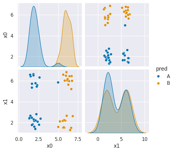
Here we see it basically predicted one side as each class because
We can repeat this experiment with several different random states:
Notebook Cell
random_state_list = [4,5,3989,37,5893859]
gnb_corners_data = []
means = []
xylim = 0
for cur_rand_state in random_state_list:
      cur_res = {'random_state':cur_rand_state}
      X_train_r, X_test_r, y_train_r, y_test_r = train_test_split(df6[['x0','x1']],df6['char'],
                                                      random_state =cur_rand_state)
      gnb.fit(X_train_r, y_train_r)
      cur_res['score'] = float(np.round(gnb.score(X_test_r,y_test_r)*100,2))
      df_sampled = pd.DataFrame(np.concatenate([np.random.multivariate_normal(th, sig*np.eye(2),N)
            for th, sig in zip(gnb.theta_,gnb.var_)]),
            columns = ['x0','x1'])
      means.append(gnb.theta_)
      df_sampled['char'] = [ci for cl in [[c]*N for c in gnb.classes_] for ci in cl]
      df_sampled['type']= 'sampled'
      df_train = X_train_r.copy()
      df_train['char'] = y_train_r
      df_train['type'] = 'train'
      df_test = X_test_r.copy()
      df_test['char'] = gnb.predict(X_test_r)
      df_test['type'] = 'pred'
      cur_res['df'] = pd.concat([df_sampled, df_train, df_test],axis=0)
      xylim = max(xylim,cur_res['df'][['x0','x1']].max().max())
      # cur_res['test_plot'] = sns.pairplot(cur_res['test'],hue='pred',hue_order=['A','B'])
      gnb_corners_data.append(cur_res)

sns.set_theme(font_scale=2)

rand_scores = {'random_state':[],
            'score':[]}
for res in gnb_corners_data:
      rand_scores['score'].append(res['score'])
      rand_scores['random_state'].append(res['random_state'])
score_df = pd.DataFrame(rand_scores)
And we can look at the sampled data, training data, and predictions for each of these differen random seed values
With random state: 4, we got a score of 72.0 %
<seaborn.axisgrid.FacetGrid at 0x7efe24ff1ee0>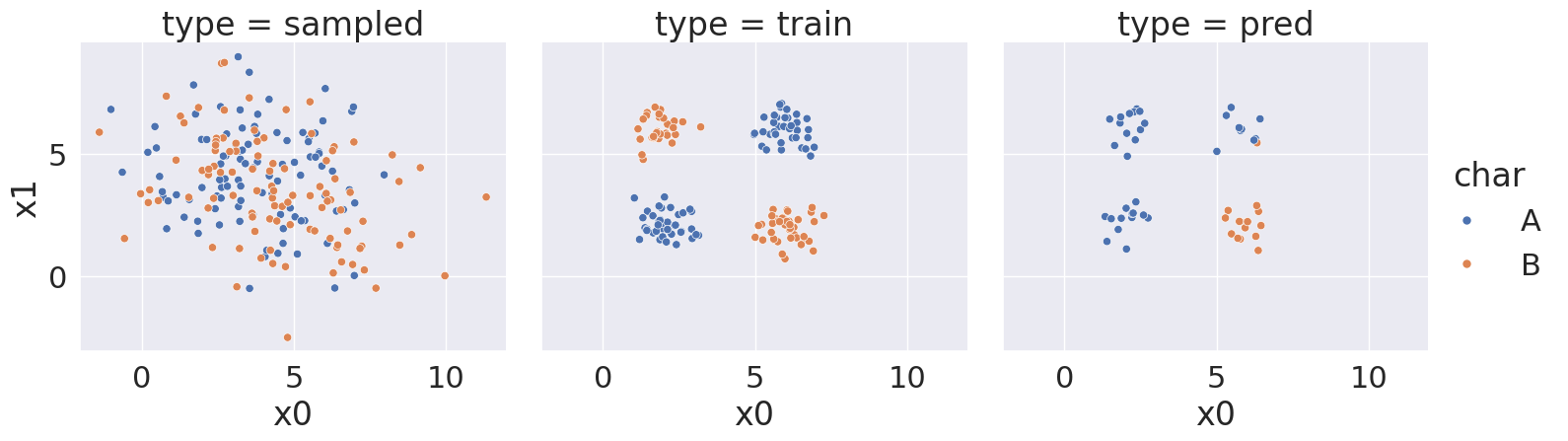
With random state: 5, we got a score of 34.0 %
<seaborn.axisgrid.FacetGrid at 0x7efe24ee1ee0>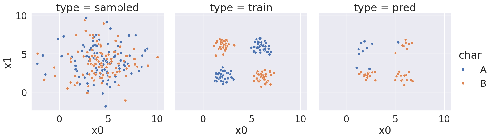
With random state:3989, we got a score of 68.0 %
<seaborn.axisgrid.FacetGrid at 0x7efe249454f0>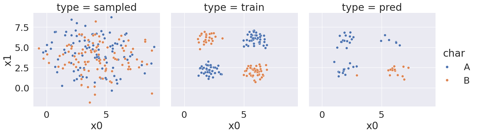
With random state: 37, we got a score of 56.0 %
<seaborn.axisgrid.FacetGrid at 0x7efe24a11f70>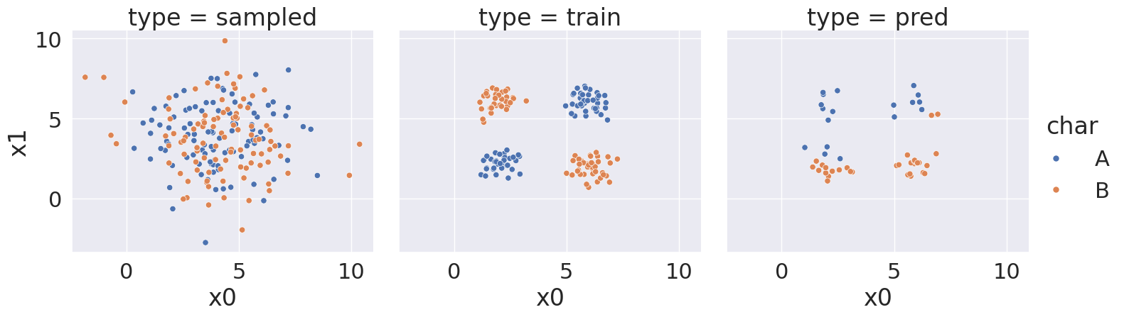
With random state: 5893859, we got a score of 56.0 %
<seaborn.axisgrid.FacetGrid at 0x7efe24853c80>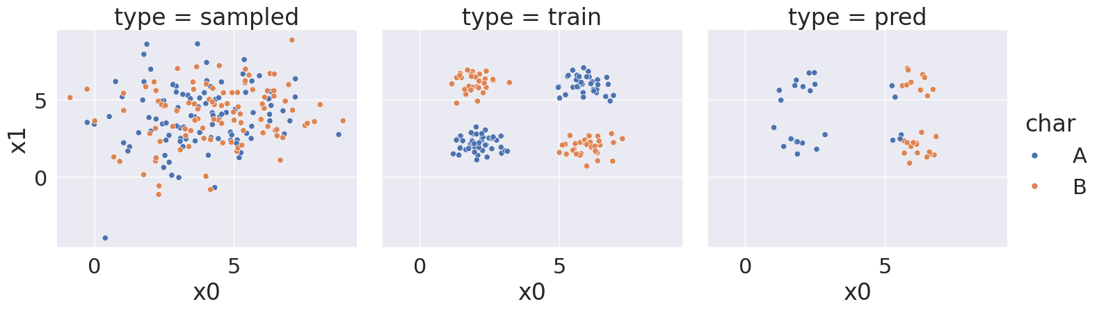
Notice that over a bunch of random splits of the data we got a variety of different solutions, but all of them have a similarity tht the means and variances are not far apart, so GaussianNB always learns basically the same representation for both classes.
Then the predictions are not very good. At most ~75% correct.
Decision Trees
This data does not fit the assumptions of the Naive Bayes model, but a decision tree has different assumptions: It basically learns a flowchart for deciding what class the sample belongs to at test time . It can be more complex, but for the scikit learn one relies on splitting the data at a series of points along one feature at a time, sequentially.
It’s only assumption is that we can make cuts along one feature at a time.
It is a discriminative model, because it describes how to discriminate (in the sense of differentiate) between the classes. This is in contrast to the generative model that describes how the data is distributed.
That said, sklearn makes using new classifiers really easy once have learned one. All of the classifiers have the same API (same methods and attributes).
Let’s instantiate the object for a decision tree.
dt = tree.DecisionTreeClassifier()and fit
dt.fit(X_train,y_train)and score
dt.score(X_test,y_test)0.94much better than the first model, that used the same random seed (67) or any of the random trials with other random seeds.
How do Decision trees make predictions
the tree module also allows you to plot the tree to examine it.
plt.figure(figsize=(15,20))
tree.plot_tree(dt, rounded =True, class_names = ['A','B'],
      proportion=True, filled =True, impurity=False,fontsize=13);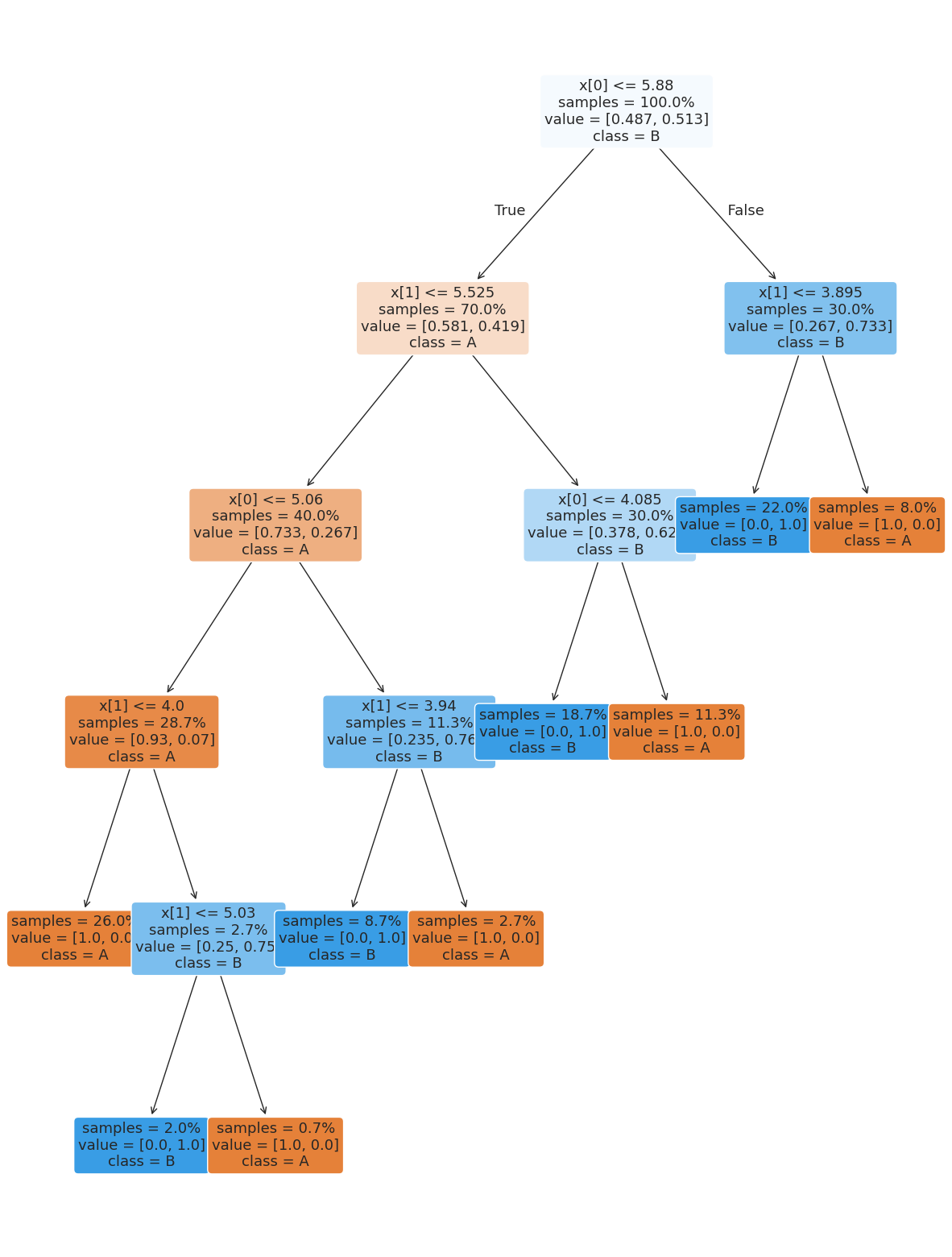
To make a prediction, once we have the tree, the algorithm follows it like a flow chart.
So for example, for the first test sample
X_test.iloc[0:1]The tree first looks at feature x0 and compares to 5.88, since it is less than that it goes to the left node (labeled True). Next it compares feature x1 to 5.525, it’s also less than that so it goes left again, then x1 to 4.0, which is also true so we go left again and then predict class A.
We can check this result:
dt.predict(X_test.iloc[0:1])array(['A'], dtype=object)Solution to Exercise 1
You can pick any value like:
my_sample_choice = 5
my_point = X_test.iloc[my_sample_choice:my_sample_choice+1]
my_pointand then go through the flow chart above (or your own)
dt.predict(my_point)array(['B'], dtype=object)as long as my_sample_choice< 50
Setting Classifier Parameters
The decision tree we had above has a lot more layers than we would expect. This is really simple data so we still got pretty good. However, the more complex the model, the more risk that it will learn something noisy about the training data that doesn’t hold up in the test set. This is called overfitting, we might also say that a classifier that is too complex does not generalize well.
Fortunately, we can control the parameters to make it find a simpler decision boundary.
max depth
One way we can do this is by setting the max_depth or the maximum number of height of the tree. The tree above has a depth of 7, but looking at the data we can see it seems like only 2 should be possible.
dt2 = tree.DecisionTreeClassifier(max_depth=2,)
dt2.fit(X_train,y_train)
dt2.score(X_test,y_test)0.76This does not do as well, we can check the training accuracy
dt2.score(X_train,y_train)0.78this is better, but not much. In general, when the test and train accuracies are close, that means a more complex model will not yet be overfitting.
We can cagain look at the tree
plt.figure(figsize=(15,20))
tree.plot_tree(dt2, rounded =True, class_names = ['A','B'],
      proportion=True, filled =True, impurity=False,fontsize=13);
We can also try one more level
dt3 = tree.DecisionTreeClassifier(max_depth=3)
dt3.fit(X_train,y_train).score(X_test,y_test)0.94This does well!
Splitting rul
The splitting rule Or make it more random:
dt2 = tree.DecisionTreeClassifier(max_depth=2,splitter='random',
                        random_state=239)
dt2.fit(X_train,y_train).score(X_test,y_test)0.86this random seed happens to do better but others do not.
plt.figure(figsize=(15,20))
tree.plot_tree(dt2, rounded =True, class_names = ['A','B'],
      proportion=True, filled =True, impurity=False,fontsize=13);
Minimum Split size
We can also set the minimum number of samples required to make a split. We can use an integer to set it in terms of number of samples or a float as a percentage.
This means that at any node with less that this percentage of the data must be a leaf node.
dt_large_split = tree.DecisionTreeClassifier(min_samples_split=.2)
dt_large_split.fit(X_train,y_train)
dt_large_split.score(X_test,y_test)0.98plt.figure(figsize=(15,20))
tree.plot_tree(dt_large_split, rounded =True, class_names = ['A','B'],
proportion=True, filled =True, impurity=False,fontsize=10);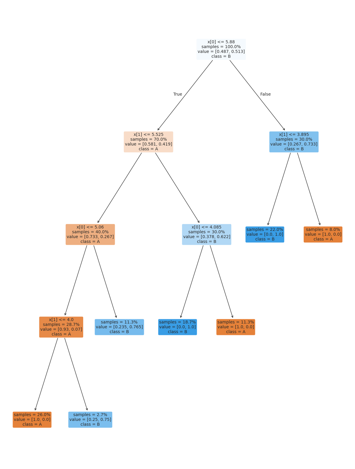
Minimum Leaf Samples
This is the number of samples that are required to make a leaf
dt_large_leaf = tree.DecisionTreeClassifier(min_samples_leaf=.2)
dt_large_leaf.fit(X_train,y_train)
dt_large_leaf.score(X_test,y_test)0.56plt.figure(figsize=(15,20))
tree.plot_tree(dt_large_leaf, rounded =True, class_names = ['A','B'],
proportion=True, filled =True, impurity=False,fontsize=10);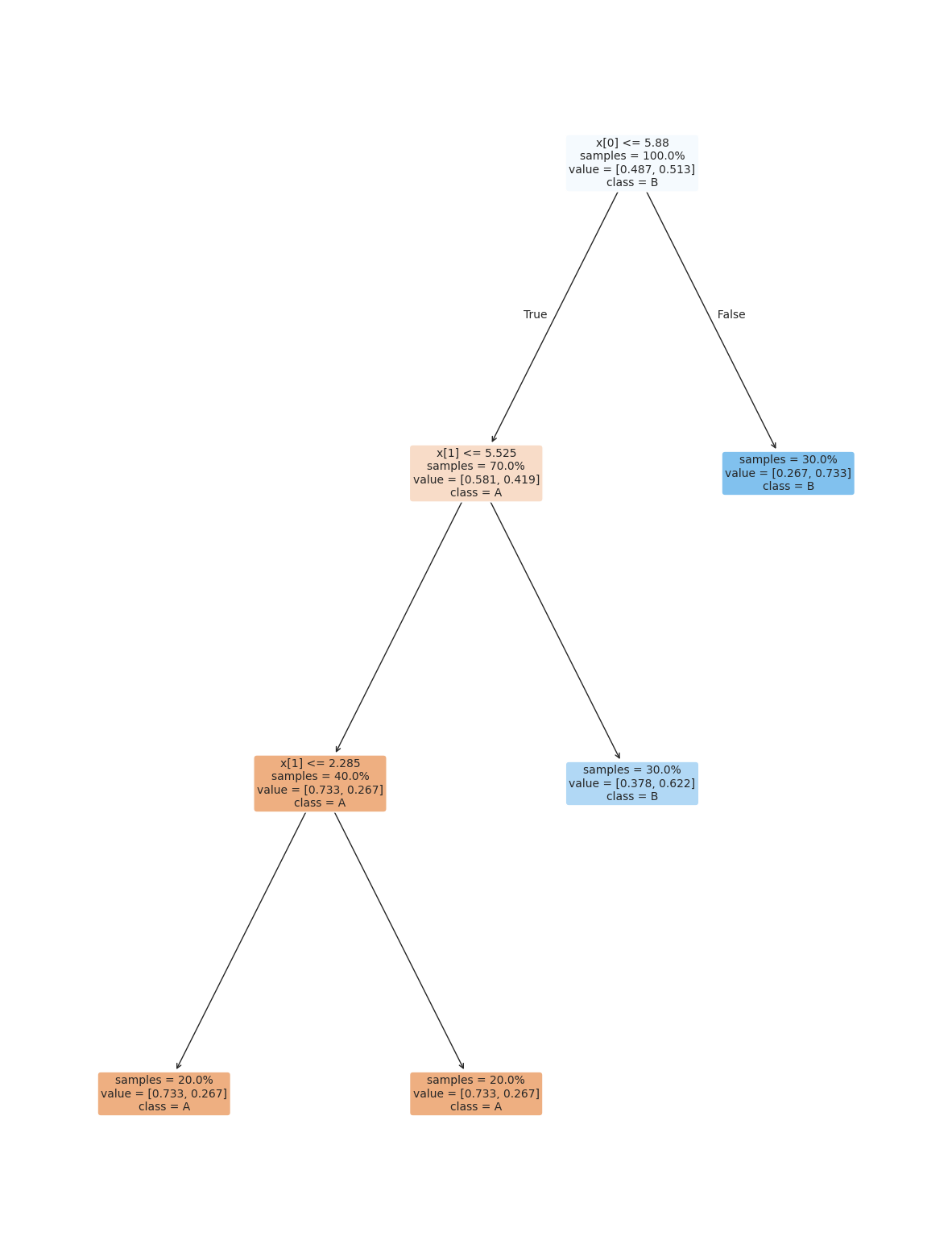
Multiple Parameters can be used together
dt_large_leaf2_d2 = tree.DecisionTreeClassifier(min_samples_split=.15,max_depth=2)
dt_large_leaf2_d2.fit(X_train,y_train)
dt_large_leaf2_d2.score(X_test,y_test)0.76plt.figure(figsize=(15,20))
tree.plot_tree(dt_large_leaf2_d2, rounded =True, class_names = ['A','B'],
proportion=True, filled =True, impurity=False,fontsize=10);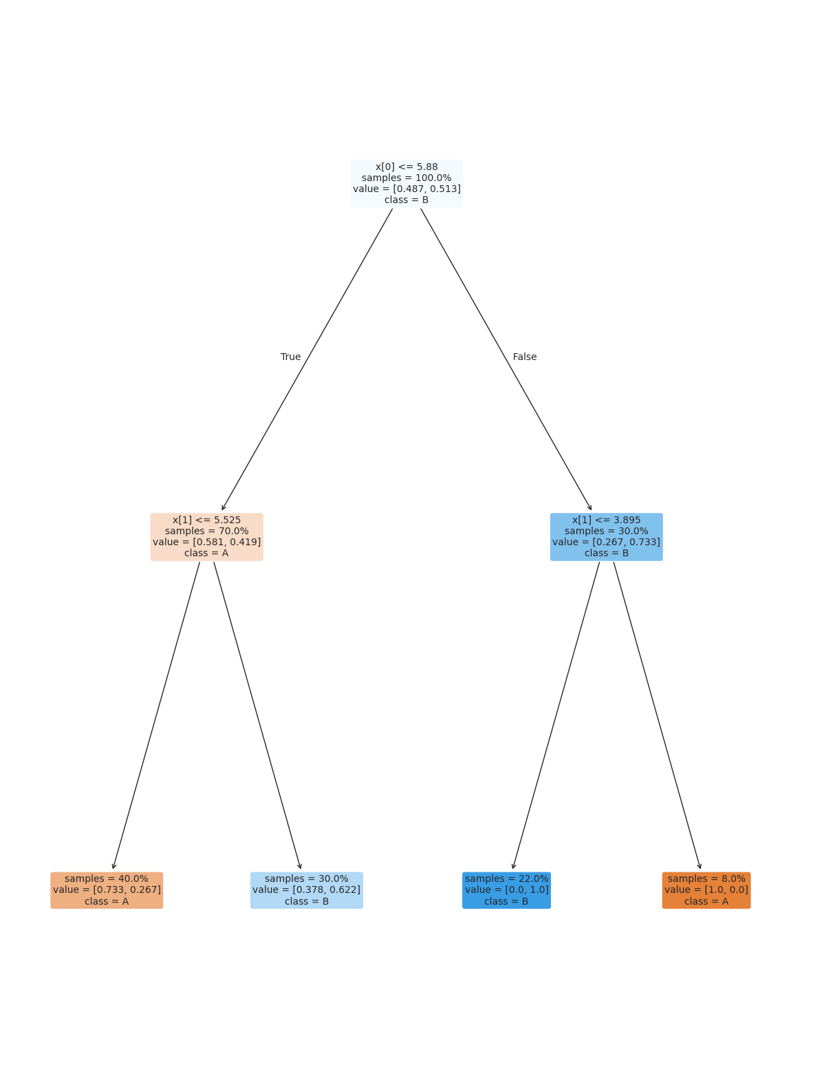
More Performance Metrics
Hint
Try to remember (or hover to look) how we got the predictions on Tuesday, when we looked at the confusion matrix
Solution to Exercise 2
y_pred = dt_large_split.predict(X_test)
print(classification_report(y_test,y_pred,labels=['A','B']))
precision recall f1-score support
A 0.97 1.00 0.98 28
B 1.00 0.95 0.98 22
accuracy 0.98 50
macro avg 0.98 0.98 0.98 50
weighted avg 0.98 0.98 0.98 50
Solution to Exercise 3
y_pred = dt_large_split.predict(X_test)
y_predA = y_pred =='A'
y_predB = y_pred =='B'
y_testA = y_test == 'A'
y_testB = y_test == 'B'
print(classification_report(y_test,y_pred,labels=['A','B']))

np.round(sum(y_pred[y_testA]==y_test[y_testA])/sum(y_testA),2)
precision recall f1-score support
A 0.97 1.00 0.98 28
B 1.00 0.95 0.98 22
accuracy 0.98 50
macro avg 0.98 0.98 0.98 50
weighted avg 0.98 0.98 0.98 50
np.float64(1.0)The overall accuracy is 98%, it has a support of 50, because there are 50[1] total samples in the test set.
For class
Athe precision is 97%, which means that 0.97[1] of the samples where it predictedA. Specifically it was correct 28 times out of 29Apredictions.For class
Bthe precision is 100%, which means that np.float64(1.0)[1] of the samples where it predictedB. Specifically it was correct 21 times out of 21Apredictions.For class
Athe recall is 100%, which means that 1.0[1] of the samples where it predictedA. Specifically it was correct 28 times out of 28 trueAsamples.For class
Bthe recall is 95%, which means that 0.95[1] of the samples where it predictedA. Specifically it was correct 21 times out of 22 trueBsamples.
For more practice, you can also go back over the notes from the COMPAS audit and try the exercises on that page.
Questions
Are there any good introductions to ScikitLearn that you are aware of?
Scikit Learn User Guide is the best one and they have a large example gallery.
Are there any popular machine learning models that use decision trees?
Yes, a lot of medical appilcations do, because since they are easy to understand, it is easier for healthcare providers to trust them.
Do predictive algorithms have pros and cons? Or is there a standard?
Each algorithm has different properties and strengths and weaknesses. Some are more popular than others, but they all do have weaknesses.
how often should we use confusion matrixes? Would it be better just to check the accuracy without one?
A confusion matrix gives more detail on the performance than accuracy alone. If the accuracy was like 99.99 maybe the confustion matrix is not informative, but otherwise, it is generally useful to understand what types of mistakes as context for how you might use/not use/ trust the model.
Due to the initial ‘shuffling’ of data: Is it possible to get a seed/shuffle of data split so that it that does much worse in a model?
Yes you can get a bad split, we will see next week a statistical technique that helps us improve this. However, the larger your dataset, the less likely this will happen, so we mostly now just get bigger and bigger datasets.
How does gnb = GaussianNB() work?
this line calls the GaussianNB class constructor method with all default paramters.
This means it creates and object of that type, we can see that like follows
gnb_ex = GaussianNB()
type(gnb_ex)sklearn.naive_bayes.GaussianNBCan you put into words, how the classification report with row A being real positive and B being negative and vise versa when looking at row B in the notes would be very muh appreicated
In the classification report, instead of treating one class as positive and one as negative overall, it treats each class as the positive class for one row. This is beacuse the report can be generated for more than two classes.
For example in the iris data:
print(classification_report(y_test,y_pred)) precision recall f1-score support
setosa 1.00 1.00 1.00 12
versicolor 0.87 0.93 0.90 14
virginica 0.91 0.83 0.87 12
accuracy 0.92 38
macro avg 0.93 0.92 0.92 38
weighted avg 0.92 0.92 0.92 38
There are 3 classes so we get a precision, recall and f1score for each of the three classes.
So the veriscolor row treats versicolor as the positive class and both the setosa and virginica as the negative class.
When do we use a decision tree?
A decision tree is a good model, when you want it to be interpretable, but do not need a generative model (we cannot generate sampels from a decision tree).
I have trouble interpreting the built-in feature of shift+tab. How can I gain a better understanding of what it means?
The shift+tab feature shows the docstring from the function.
there is a pep[2] for docstrings
the pep8 guide might help
most scientific computing docstrings are numpydoc style (example spec)