Model Comparison

To compare models, we will first optimize the parameters of two diffrent models and look at how the different parameters settings impact the model comparison. Later, we’ll see how to compare across models of different classes.

We can compare models along several dimensions:

• model performance (metrics like accuracy, $R^2$, Kmeans objective, disparate impact, equal opportunity difference, precision or recall)

• interpretability

• generative vs discriminative

• adherance to model assumptions

• time/cost to run

• amount of features required

Fitting models to compare¶

import matplotlib.pyplot as plt
import numpy as np
import seaborn as sns
import pandas as pd
from sklearn import datasets
from sklearn import cluster
from sklearn import svm
from sklearn import tree
from sklearn import naive_bayes
# import the whole model selection module
from sklearn import model_selection
sns.set_theme(palette='colorblind')

We’ll use the iris data again.

Remember, we need to split the data into training and test. The cross validation step will hep us optimize the parameters, but we don’t want data leakage where the model has seen the test data multiple times. So, we split the data here for train and test and the cross validation splits the training data into train and “test” again, but that “test” is better termed validation.

# load and split the data
iris_X, iris_y = datasets.load_iris(return_X_y=True)
iris_X_train, iris_X_test, iris_y_train, iris_y_test = model_selection.train_test_split(
    iris_X,iris_y, test_size =.2,random_state=5)

cv = 5

Next, we’ll create some variables for the sizes of these sets of data so that we can use them later

num_test = len(iris_y_test)
num_val = len(iris_y_train)/cv

Fitting a Decision Tree¶

We will first fit a decision tree.

Then we can make the object, the parameter grid dictionary and the Grid Search object. We split these into separate cells, so that we can use the built in help to see more detail.

# create dt, set param grid & create optimizer
dt = tree.DecisionTreeClassifier()

params_dt = {'criterion':['gini','entropy'],
             'max_depth':[2,3,4,5,6],
       'min_samples_leaf':list(range(2,20,2))}

dt_opt = model_selection.GridSearchCV(dt,params_dt,cv=cv)


# optimize the decision tree
dt_opt.fit(iris_X_train,iris_y_train)

# store dt optimization
dt_df = pd.DataFrame(dt_opt.cv_results_)

GNB¶

We’ll also fit GNB, it doesn’t really have parameters to optmize, but we will use the optimizer to run the experiment so we have the score times evaluated in the same way as the others.

# create dt, set param grid & create optimizer
gnb = naive_bayes.GaussianNB()

params_gnb = {'priors':[[.33,.34,.33]],}

gb_opt = model_selection.GridSearchCV(gnb,params_gnb,cv=cv)


# optimize the decision tree
gb_opt.fit(iris_X_train,iris_y_train)

# store dt optimization
gb_df = pd.DataFrame(gb_opt.cv_results_)

Support Vector Machine¶

Third, we will use a new type of classifier.

A support vector machine or SVM is a type of maximum margin classifier. That is it tries to find the decision boundary that produces the clearest margin.

You can see a visualization of the impact of the C parameter in alinear model

Source

# we create 40 separable points
np.random.seed(0)
X = np.r_[np.random.randn(20, 2) - [2, 2], np.random.randn(20, 2) + [2, 2]]
Y = [0] * 20 + [1] * 20

# figure number
fignum = 1

# fit the model
for name, penalty in (("unreg", 1),):
    clf = svm.SVC(kernel="linear", C=penalty)
    clf.fit(X, Y)

    # get the separating hyperplane
    w = clf.coef_[0]
    a = -w[0] / w[1]
    xx = np.linspace(-5, 5)
    yy = a * xx - (clf.intercept_[0]) / w[1]

    # plot the parallels to the separating hyperplane that pass through the
    # support vectors (margin away from hyperplane in direction
    # perpendicular to hyperplane). This is sqrt(1+a^2) away vertically in
    # 2-d.
    margin = 1 / np.sqrt(np.sum(clf.coef_**2))
    yy_down = yy - np.sqrt(1 + a**2) * margin
    yy_up = yy + np.sqrt(1 + a**2) * margin

    # plot the line, the points, and the nearest vectors to the plane
    plt.figure(fignum, figsize=(4, 3))
    plt.clf()
    plt.plot(xx, yy, "k-")
    plt.plot(xx, yy_down, "k--")
    plt.plot(xx, yy_up, "k--")

    plt.scatter(
        clf.support_vectors_[:, 0],
        clf.support_vectors_[:, 1],
        s=80,
        facecolors="none",
        zorder=10,
        edgecolors="k",
    )
    plt.scatter(
        X[:, 0], X[:, 1], c=Y, zorder=10, cmap=plt.get_cmap("RdBu"), edgecolors="k"
    )

    plt.axis("tight")
    x_min = -4.8
    x_max = 4.2
    y_min = -6
    y_max = 6

    YY, XX = np.meshgrid(yy, xx)
    xy = np.vstack([XX.ravel(), YY.ravel()]).T
    Z = clf.decision_function(xy).reshape(XX.shape)

    # Put the result into a contour plot
    plt.contourf(XX, YY, Z, cmap=plt.get_cmap("RdBu"), alpha=0.5, linestyles=["-"])

    plt.xlim(x_min, x_max)
    plt.ylim(y_min, y_max)

    plt.xticks(())
    plt.yticks(())
    fignum = fignum + 1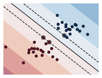

We can fit and optimize it the same way as others

#  creat svm and optimizer
svm_clf = svm.SVC()
param_grid = {'kernel':['linear','rbf'], 'C':[.05, .25, .5, .75,1,2,5,7,10]}
svm_opt = model_selection.GridSearchCV(svm_clf,param_grid,cv=cv)

# fit the model and  put the CV results in a dataframe
svm_opt.fit(iris_X_train,iris_y_train)
sv_df = pd.DataFrame(svm_opt.cv_results_)

Comparing the models¶

Validation scores¶

First we will look at the validation scores:

dt_opt.best_score_, gb_opt.best_score_, svm_opt.best_score_

These scores are aall pretty high, and remember, they are the average of scoring 24.0 samples in the validation set 5 times.

Test accuracy¶

Since the validation sets are used to pick the best hyperparameters for each model, a better measure of performance is the true test accuracy.

dt_opt.best_estimator_.score(iris_X_test,iris_y_test)

gb_opt.best_estimator_.score(iris_X_test,iris_y_test)

svm_opt.best_estimator_.score(iris_X_test,iris_y_test)

These are a little lower than the validation scores. They’re still all pretty close, especially since the test set is not that big (30)

Parameter Sensitivity¶

Remember, however, that the grid search tries a lot of parameter settings. We can look at how much the performance depends on the values of the parameters.

dt_df['mean_test_score'].describe()

sv_df['mean_test_score'].describe()

A lower std might signal that the model does not care about the parameters and might generalize better. A higher minimum score is also a good sign, in this same vein.

For GNB we can look but, there is only one parameter setting so it is not dependent

gb_df['mean_test_score'].describe()

Confidence Intervals¶

def classification_confint(acc,n):
    '''
    Compute the 95% confidence interval for a classification problem.

    Parameters
    ----------
    acc : float
       classification accuracy in [0,1]
    n : int
     number of observations used to compute the accuracy (test set size)

    Returns
    --------
    bounds: tuple 
        (lb,ub) the lower and upper bounds of the interval
    '''
    interval = 1.96*np.sqrt(acc*(1-acc)/n)
    lb = max(0, acc - interval)
    ub = min(1.0, acc + interval)
    return (lb,ub)

Despite the warnings, this still provides a good rough intuition for checking if the difference between two performances.

svm_acc = svm_opt.best_estimator_.score(iris_X_test,iris_y_test)
dt_acc = dt_opt.best_estimator_.score(iris_X_test,iris_y_test)
gnb_acc  = gb_opt.best_estimator_.score(iris_X_test,iris_y_test)

We can then compute the intervals for the three models:

classification_confint(svm_acc,num_test)

classification_confint(dt_acc,num_test)

classification_confint(gnb_acc,num_test)

These all overlap, so the differences are not statistically significantly different. Meaning, statistically, none are better, given the assumptions of this test.

Let’s imagine we had a lot more test samples: ,

classification_confint(svm_acc,num_test*10)

classification_confint(dt_acc,num_test*10)

classification_confint(gnb_acc,num_test*10)

the intervals get narrower and then the SVM interval no longer overlaps the other two. So, if we had a lot more samples in the test set and got the same accuracy, then we could say the SVM was better.

We can also use this to plot how wide the interval is for different size test sets.

acc=.95
n_list = list(range(1,200))
intervals = [1.96*np.sqrt(acc*(1-acc)/n) for n in n_list]
plt.plot(n_list, intervals)
plt.xlabel('test set size')
plt.ylabel('interval width')
#highlight a point for discussion

ex_pt = 49
ex_samples = n_list[ex_pt]
ex_interval = intervals[ex_pt]
plt.plot(ex_samples, ex_interval,'or')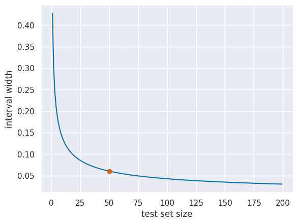

To read this, the highlighted point, for example, means that for 50 samples in the test set the difference in accuracy needs to be at least 6.04% for it to be significant.

Questions¶

Is there a final exam?¶

No scheduled exam. You will only need to add to and extend your portfolio, due on the day of our scheduled exam(to read that, look for TR 3:30, which is when our class meets, that is in the Thursday December 11 row)

How do the parameters affect the scores?¶

In general the parameters change which final model the fit algorithm finds. The splits and their order in a decision tree; the specific decision boundary in an SVM; the number of features used in LASSO; etc.

More specifically, this varies by dataset. Answering this question thoroughly is a way to earn innovative.