4. Exploratory Data Analysis

Now we get to start actual data science!

4.1. This week: Exploratory Data Analysis

• How to summarize data

• Interpretting summaries

• Visualizing data

• interpretting summaries

4.1.1. Summarizing and Visualizing Data are very important

• People cannot interpret high dimensional or large samples quickly

• Important in EDA to help you make decisions about the rest of your analysis

• Important in how you report your results

• Summaries are similar calculations to performance metrics we will see later

• visualizations are often essential in debugging models

THEREFORE

• You have a lot of chances to earn summarize and visualize

• we will be picky when we assess if you earned them or not

import pandas as pd

Today we will work with a new dataset about Carbon emissions

carbon_data_url = 'https://github.com/rfordatascience/tidytuesday/raw/master/data/2024/2024-05-21/emissions.csv'

carbon_df = pd.read_csv(carbon_data_url)

data readme

carbon_df.head()

	year	parent_entity	parent_type	commodity	production_value	production_unit	total_emissions_MtCO2e
0	1962	Abu Dhabi National Oil Company	State-owned Entity	Oil & NGL	0.91250	Million bbl/yr	0.363885
1	1962	Abu Dhabi National Oil Company	State-owned Entity	Natural Gas	1.84325	Bcf/yr	0.134355
2	1963	Abu Dhabi National Oil Company	State-owned Entity	Oil & NGL	1.82500	Million bbl/yr	0.727770
3	1963	Abu Dhabi National Oil Company	State-owned Entity	Natural Gas	4.42380	Bcf/yr	0.322453
4	1964	Abu Dhabi National Oil Company	State-owned Entity	Oil & NGL	7.30000	Million bbl/yr	2.911079

In this case, head shows that these rows are very similar because it is sorted. Tail would probably be similar, so we will try sample to get a random subset.

carbon_df.sample(5)

	year	parent_entity	parent_type	commodity	production_value	production_unit	total_emissions_MtCO2e
6827	1995	North Korea	Nation State	Anthracite Coal	13.221050	Million tonnes/yr	38.574888
1591	2018	Canadian Natural Resources	Investor-owned Company	Oil & NGL	299.665000	Million bbl/yr	119.499778
1166	2009	BHP	Investor-owned Company	Metallurgical Coal	36.416000	Million tonnes/yr	108.032327
9007	2015	Poland	Nation State	Metallurgical Coal	12.985117	Million tonnes/yr	38.521870
11088	1999	Suncor Energy	Investor-owned Company	Natural Gas	393.800000	Bcf/yr	28.704236

4.2. Describing a Dataset

So far, we’ve loaded data in a few different ways and then we’ve examined DataFrames as a data structure, looking at what different attributes they have and what some of the methods are, and how to get data into them.

The describe method provides us with a set of summary statistics that broadly

further reading

On the documentation page for describe the “ See Also” shows the links to the documentation of most of the individual functions. This is a good way to learn about other things, or find something when you are not quite sure what it would be named. Go to a function thats similar to what you want and then look at the related functions.

carbon_df.describe()

	year	production_value	total_emissions_MtCO2e
count	12551.000000	12551.000000	12551.000000
mean	1987.148116	412.712258	113.219734
std	29.202455	1357.569683	329.812666
min	1854.000000	0.004398	0.000321
25%	1973.000000	10.601353	8.785294
50%	1994.000000	63.203536	33.058688
75%	2009.000000	320.664764	102.154596
max	2022.000000	27192.000000	8646.905949

And these all give us a sense of the values and the distribution or spread fo the data in each column.

4.2.1. Individual statistics

We can also extract each of the statistics that the describe method calculates individually, by name.

carbon_df.max()

year                                    2022
parent_entity                            YPF
parent_type               State-owned Entity
commodity                       Thermal Coal
production_value                     27192.0
production_unit            Million tonnes/yr
total_emissions_MtCO2e           8646.905949
dtype: object

4.2.2. Understanding Quantiles

The 50% has another more common name: the median. It means 50% of the data are lower (and higher) than this value.

The quantiles are tricky, we cannot just .25%() to get the 25% percentile, we have to use the quantile method and pass it a value between 0 and 1.

carbon_df['production_value'].quantile(.25)

10.6013534253315

carbon_df['production_value'].quantile(.8)

448.5

4.3. Individual variable

We can use the descriptive statistics on individual columns as well

4.4. What is the average total emissions in this dataset?

carbon_df['total_emissions_MtCO2e'].mean()

113.21973391166483

4.5. Working with categorical data

There are different columns in the describe than the the whole dataset:

carbon_df.columns

Index(['year', 'parent_entity', 'parent_type', 'commodity', 'production_value',
       'production_unit', 'total_emissions_MtCO2e'],
      dtype='object')

So far, the stats above are only for numerical features.

We can get the prevalence of each one with value_counts, this can also allow us to answer certain questions. Let’s try a few.

4.5.1. What is the most common parent type?

carbon_df['parent_type'].value_counts()

parent_type
Investor-owned Company    6583
State-owned Entity        3914
Nation State              2054
Name: count, dtype: int64

Hint

This file works as a notebook, that gets run when the HTML is built for the site. Here, I used the glue feature to use a value from the code cell in the markdown

Show code cell source Hide code cell source

from myst_nb import glue
most_common_ptype = carbon_df['parent_type'].value_counts().idxmax()
glue('max_parent',most_common_ptype)

'Investor-owned Company'

This shows us that the most common one is ‘Investor-owned Company’

We also notice that the data is relatively balanced enough that we can make good comparisons from the overall output.

For the specific question, we could instead use the mode method (the most frequent value).

carbon_df['parent_type'].mode()

0    Investor-owned Company
Name: parent_type, dtype: object

4.5.2. Is it reasonable to compare and use all of the the commodity types in the data

To do this, we again look at the value counts:

carbon_df['commodity'].value_counts()

commodity
Oil & NGL              3733
Natural Gas            3452
Bituminous Coal        1370
Metallurgical Coal     1073
Lignite Coal           1008
Sub-Bituminous Coal     673
Thermal Coal            611
Anthracite Coal         368
Cement                  263
Name: count, dtype: int64

Here, we note that the top few are a lot more similar and the smallest one is a lot lower. Here we might drop only the bottom couple or keep them call becaus for a lot of things 200 measurements is enough.

Another choice is that we could combine the different types of coals together. We can do this by adding a column.

carbon_df['commodity_simple'] = carbon_df['commodity'].apply(lambda s: s if not('Coal' in s) else 'Coal')

The way this works is:

• carbon_df['commodity'] picks out the column of interest

• the .apply method applies a function (that we pass to it) to all of the elements of a series (or to the rows or columns of a DataFrame)

• lambda s: s if not('Coal' in s) else 'Coal' is a lambda function that returns the same value if Col is not in it or only Coal if it is

• assigns values to a column 'commodity_simple' carbon_df['commodity_simple'] =. It also creates that column since it did not exist

4.5.3. understanding lambda functions

To better understand the lambda function that we used above, let’s assign it to a variable.

coal_strip = lambda s: s if not('Coal' in s) else 'Coal'

First we will inspect it a little:

type(coal_strip)

function

We can see it is a function here

Now we can make calls to it, like any other functions

coal_strip('Metallurgical Coal')

'Coal'

this works and now we test the other case:

coal_strip('naything else')

'naything else'

4.5.4. How a column is added

Now we can see a sample of the DataFrame again to see how the apply method works.

carbon_df.sample(5)

	year	parent_entity	parent_type	commodity	production_value	production_unit	total_emissions_MtCO2e	commodity_simple
8908	1996	Poland	Nation State	Lignite Coal	63.845576	Million tonnes/yr	85.502641	Coal
4276	1903	ExxonMobil	Investor-owned Company	Natural Gas	17.322720	Bcf/yr	1.262660	Natural Gas
8412	1992	Petroleum Development Oman	State-owned Entity	Natural Gas	145.655315	Bcf/yr	10.616873	Natural Gas
4248	2020	Exxaro Resources Ltd	Investor-owned Company	Metallurgical Coal	5.331660	Million tonnes/yr	15.816993	Coal
9694	2022	Russian Federation	Nation State	Metallurgical Coal	98.936523	Million tonnes/yr	293.506779	Coal

We can further examine this column:

carbon_df['commodity_simple'].value_counts()

commodity_simple
Coal           5103
Oil & NGL      3733
Natural Gas    3452
Cement          263
Name: count, dtype: int64

Now the numbers are more similar, we might want to drop the cement, we can do that using a mask that we saw last week.

4.6. Split-Apply-Combine

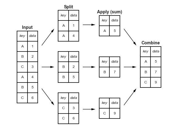
see it in action on pandas tutor

4.6.1. Which commodity type has the highest average emissions?

To do this we group by the categorical value, the new simplified commodity column we created, then we pick out thee emissions column, and take the average.

carbon_df.groupby('commodity_simple')['total_emissions_MtCO2e'].mean()

commodity_simple
Cement         112.859242
Coal           118.369779
Natural Gas     75.073875
Oil & NGL      141.479481
Name: total_emissions_MtCO2e, dtype: float64

4.6.2. How apply works

We can use apply with any function, that we write in advance, that comes from a library, or is built in. Above, we used a lambda we defined on the fly, but here we can make it first.

def first_chars(s):
  return s[:5]

carbon_df['commodity'].apply(first_chars)

0        Oil &
1        Natur
2        Oil &
3        Natur
4        Oil &
         ...  
12546    Natur
12547    Oil &
12548    Natur
12549    Oil &
12550    Natur
Name: commodity, Length: 12551, dtype: object

4.6.3. Grouping Multiple times

we can pass a list to group by two values

carbon_df.groupby(['commodity_simple','parent_type'])['total_emissions_MtCO2e'].mean()

commodity_simple  parent_type           
Cement            Investor-owned Company     38.813769
                  Nation State              243.802816
Coal              Investor-owned Company     45.397065
                  Nation State              228.621342
                  State-owned Entity         94.977580
Natural Gas       Investor-owned Company     58.313678
                  Nation State              741.445688
                  State-owned Entity         80.152170
Oil & NGL         Investor-owned Company    106.583580
                  Nation State              885.428265
                  State-owned Entity        162.042650
Name: total_emissions_MtCO2e, dtype: float64

This is one Series, but is has a multi-index. We can check the type

em_by_comm_parent = carbon_df.groupby(['commodity_simple','parent_type'])['total_emissions_MtCO2e'].mean()
type(em_by_comm_parent)

pandas.core.series.Series

and look at the index to confirm

em_by_comm_parent.index

MultiIndex([(     'Cement', 'Investor-owned Company'),
            (     'Cement',           'Nation State'),
            (       'Coal', 'Investor-owned Company'),
            (       'Coal',           'Nation State'),
            (       'Coal',     'State-owned Entity'),
            ('Natural Gas', 'Investor-owned Company'),
            ('Natural Gas',           'Nation State'),
            ('Natural Gas',     'State-owned Entity'),
            (  'Oil & NGL', 'Investor-owned Company'),
            (  'Oil & NGL',           'Nation State'),
            (  'Oil & NGL',     'State-owned Entity')],
           names=['commodity_simple', 'parent_type'])

We can use reset_index to change from the multi-index into a new count from 0 index (and make it a DataFrame in the process)

carbon_df.groupby(['commodity_simple','parent_type'])['total_emissions_MtCO2e'].mean().reset_index()

	commodity_simple	parent_type	total_emissions_MtCO2e
0	Cement	Investor-owned Company	38.813769
1	Cement	Nation State	243.802816
2	Coal	Investor-owned Company	45.397065
3	Coal	Nation State	228.621342
4	Coal	State-owned Entity	94.977580
5	Natural Gas	Investor-owned Company	58.313678
6	Natural Gas	Nation State	741.445688
7	Natural Gas	State-owned Entity	80.152170
8	Oil & NGL	Investor-owned Company	106.583580
9	Oil & NGL	Nation State	885.428265
10	Oil & NGL	State-owned Entity	162.042650

4.7. Prepare for next class

Seaborn is a plotting library that gives us opinionated defaults

Important

Run this line one time before class on Thursday

import seaborn as sns

If you get ModuleNotFound error, open a terminal tab and run pip install seaborn .

seaborn’s alias is sns as an inside joke among the developers to the character, Samual Norman Seaborn from West Wing they named the library after per their FAQ

4.8. Questions After Class

Important

Questions about the assignment have been addreessed by adding hints and tips to the end of the instructions

4.8.1. when putting the two column names ["commodity_simple", "parent_type"] in the square brackets, what did that do?

We cann answer a question like this by inspecting the code further

First we can look directly at it:

["commodity_simple", "parent_type"]

['commodity_simple', 'parent_type']

Next, we can check its type:

type(["commodity_simple", "parent_type"])

list

It makes a list which is then compatible with the groupby method.

We can look a its help to remember what it can be passed:

# the __doc__ attribute is a property of all functions
# it is a string so I used split to break it into lines, 
# looked to see how many i needed then joined them back together
# and printed them (to have the newkines render)
print('\n'.join(carbon_df.groupby.__doc__.split('\n')[:18]))

Group DataFrame using a mapper or by a Series of columns.

A groupby operation involves some combination of splitting the
object, applying a function, and combining the results. This can be
used to group large amounts of data and compute operations on these
groups.

Parameters
----------
by : mapping, function, label, pd.Grouper or list of such
    Used to determine the groups for the groupby.
    If ``by`` is a function, it's called on each value of the object's
    index. If a dict or Series is passed, the Series or dict VALUES
    will be used to determine the groups (the Series' values are first
    aligned; see ``.align()`` method). If a list or ndarray of length
    equal to the selected axis is passed (see the `groupby user guide
    <https://pandas.pydata.org/pandas-docs/stable/user_guide/groupby.html#splitting-an-object-into-groups>`_),

4.8.2. How does the apply function work?

I have explained it and linked resources above, plus the pandas docs have a section on it in their user guide

4.8.3. How should we be practicing this material. Its hard to tell whats the specific take away from this class vs memorizing methods.

Review the notes and see the analysis.

What we did is ann example data anlysis. We asked and answered several questions. This serves as example questions and types of questions. How to interpret the statistics.

4.8.4. what does the lambda do inside of the function we created to group the coal commodity

lambda is the keyword to define a function in line, like def is in a full length definition.

4.8.5. Is there a way to scrape data from a website and make it a csv file if the website does not allow for exporting?

Sometimes, we will learn webscraping in a few weeks. For now, download locally, or try a different dataset.

4.8.6. Will be working on forms of data visualization?

Yes