14. Clustering#
Clustering is unsupervised learning. That means we do not have the labels to learn from. We aim to learn both the labels for each point and some way of characterizing the classes at the same time.
Computationally, this is a harder problem. Mathematically, we can typically solve problems when we have a number of equations equal to or greater than the number of unknowns. For \(N\) data points ind \(d\) dimensions and \(K\) clusters, we have \(N\) equations and \(N + K*d\) unknowns. This means we have a harder problem to solve.
For today, we’ll see K-means clustering which is defined by \(K\) a number of clusters and a mean (center) for each one. There are other K-centers algorithms for other types of centers.
Clustering is a stochastic (random) algorithm, so it can be a little harder to debug the models and measure performance. For this reason, we are going to lootk a little more closely at what it actually does than we did with classification.
14.1. KMeans#
clustering goal: find groups of samples that are similar
k-means assumption: a fixed number (\(k\)) of means will describe the data enough to find the groups
Note
This is also a naive and gaussian assumption, but it is one step stronger in that it assumes that every feature has the same covariance
14.2. Clustering with Sci-kit Learn#
import seaborn as sns
import numpy as np
from sklearn import datasets
from sklearn.cluster import KMeans
from sklearn import metrics
import pandas as pd
import matplotlib.pyplot as plt
sns.set_theme(palette='colorblind')

# set global random seed so that the notes are the same each time the site builds
np.random.seed(1103)
Today we will load the iris data from seaborn:
iris_df = sns.load_dataset('iris')
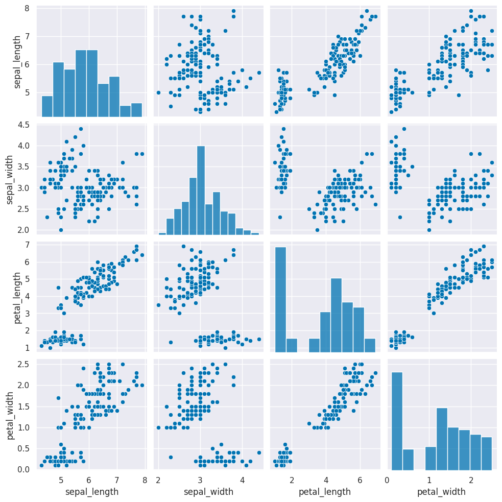
this is how the clustering algorithm sees the data, with no labels:
sns.pairplot(iris_df)
<seaborn.axisgrid.PairGrid at 0x7f6e44b0fb80>
Next we need to create a copy of the data that’s appropriate for clustering. Remember that clustering is unsupervised so it doesn’t have a target variable. We also can do clustering on the data with or without splitting into test/train splits, since it doesn’t use a target variable, we can evaluate how good the clusters it finds are on the actual data that it learned from.
We can either pick the measurements out or drop the species column. remember most data frame operations return a copy of the dataframe.
We will drop here:
iris_X = iris_df.drop(columns=['species'])
and inspect to see it:
iris_X.head()
| sepal_length | sepal_width | petal_length | petal_width | |
|---|---|---|---|---|
| 0 | 5.1 | 3.5 | 1.4 | 0.2 |
| 1 | 4.9 | 3.0 | 1.4 | 0.2 |
| 2 | 4.7 | 3.2 | 1.3 | 0.2 |
| 3 | 4.6 | 3.1 | 1.5 | 0.2 |
| 4 | 5.0 | 3.6 | 1.4 | 0.2 |
Next, we create a Kmeans estimator object with 3 clusters, since we know that the iris data has 3 species of flowers. We refer to these three groups as classes in classification (the goal is to label the classes…) and in clustering we sometimes borrow that word. Sometimes, clustering literature will be more abstract and refer to partitions, this is especially common in more mathematical/statistical work as opposed to algorithmic work on clustering.
km = KMeans(n_clusters=3)
We dropped the column that tells us which of the three classes that each sample(row) belongs to. We still have data from three species of flows.
We can use fit again, but this time it only requires the features, no labels.
km.fit(iris_X)
/opt/hostedtoolcache/Python/3.8.18/x64/lib/python3.8/site-packages/sklearn/cluster/_kmeans.py:1416: FutureWarning: The default value of `n_init` will change from 10 to 'auto' in 1.4. Set the value of `n_init` explicitly to suppress the warning
  super()._check_params_vs_input(X, default_n_init=10)
KMeans(n_clusters=3)In a Jupyter environment, please rerun this cell to show the HTML representation or trust the notebook.
On GitHub, the HTML representation is unable to render, please try loading this page with nbviewer.org.
KMeans(n_clusters=3)
We see it learns similar, but fewer, parameters:
km.__dict__
{'n_clusters': 3,
 'init': 'k-means++',
 'max_iter': 300,
 'tol': 0.0001,
 'n_init': 'warn',
 'verbose': 0,
 'random_state': None,
 'copy_x': True,
 'algorithm': 'lloyd',
 'feature_names_in_': array(['sepal_length', 'sepal_width', 'petal_length', 'petal_width'],
       dtype=object),
 'n_features_in_': 4,
 '_tol': 0.00011356176666666667,
 '_n_init': 10,
 '_algorithm': 'lloyd',
 '_n_threads': 2,
 'cluster_centers_': array([[5.006     , 3.428     , 1.462     , 0.246     ],
        [5.9016129 , 2.7483871 , 4.39354839, 1.43387097],
        [6.85      , 3.07368421, 5.74210526, 2.07105263]]),
 '_n_features_out': 3,
 'labels_': array([0, 0, 0, 0, 0, 0, 0, 0, 0, 0, 0, 0, 0, 0, 0, 0, 0, 0, 0, 0, 0, 0,
        0, 0, 0, 0, 0, 0, 0, 0, 0, 0, 0, 0, 0, 0, 0, 0, 0, 0, 0, 0, 0, 0,
        0, 0, 0, 0, 0, 0, 1, 1, 2, 1, 1, 1, 1, 1, 1, 1, 1, 1, 1, 1, 1, 1,
        1, 1, 1, 1, 1, 1, 1, 1, 1, 1, 1, 2, 1, 1, 1, 1, 1, 1, 1, 1, 1, 1,
        1, 1, 1, 1, 1, 1, 1, 1, 1, 1, 1, 1, 2, 1, 2, 2, 2, 2, 1, 2, 2, 2,
        2, 2, 2, 1, 1, 2, 2, 2, 2, 1, 2, 1, 2, 1, 2, 2, 1, 1, 2, 2, 2, 2,
        2, 1, 2, 2, 2, 2, 1, 2, 2, 2, 1, 2, 2, 2, 1, 2, 2, 1], dtype=int32),
 'inertia_': 78.851441426146,
 'n_iter_': 6}
Hint
use shift+tab or another jupyter help to figure out what the parameter names are for any function or class you’re working with.
Since we don’t have separate test and train data, we can use the fit_predict method. This is what the kmeans algorithm always does anyway, it both learns the means and the assignment (or prediction) for each sample at the same time.
This gives the labeled cluster by index, or the assignment, of each point.
If we run that a few times, we will see different solutions each time because the algorithm is random, or stochastic.
These are similar to the outputs in classification, except that in classification, it’s able to tell us a specific species for each. Here it can only say clust 0, 1, or 2. It can’t match those groups to the species of flower.
14.3. Visualizing the outputs#
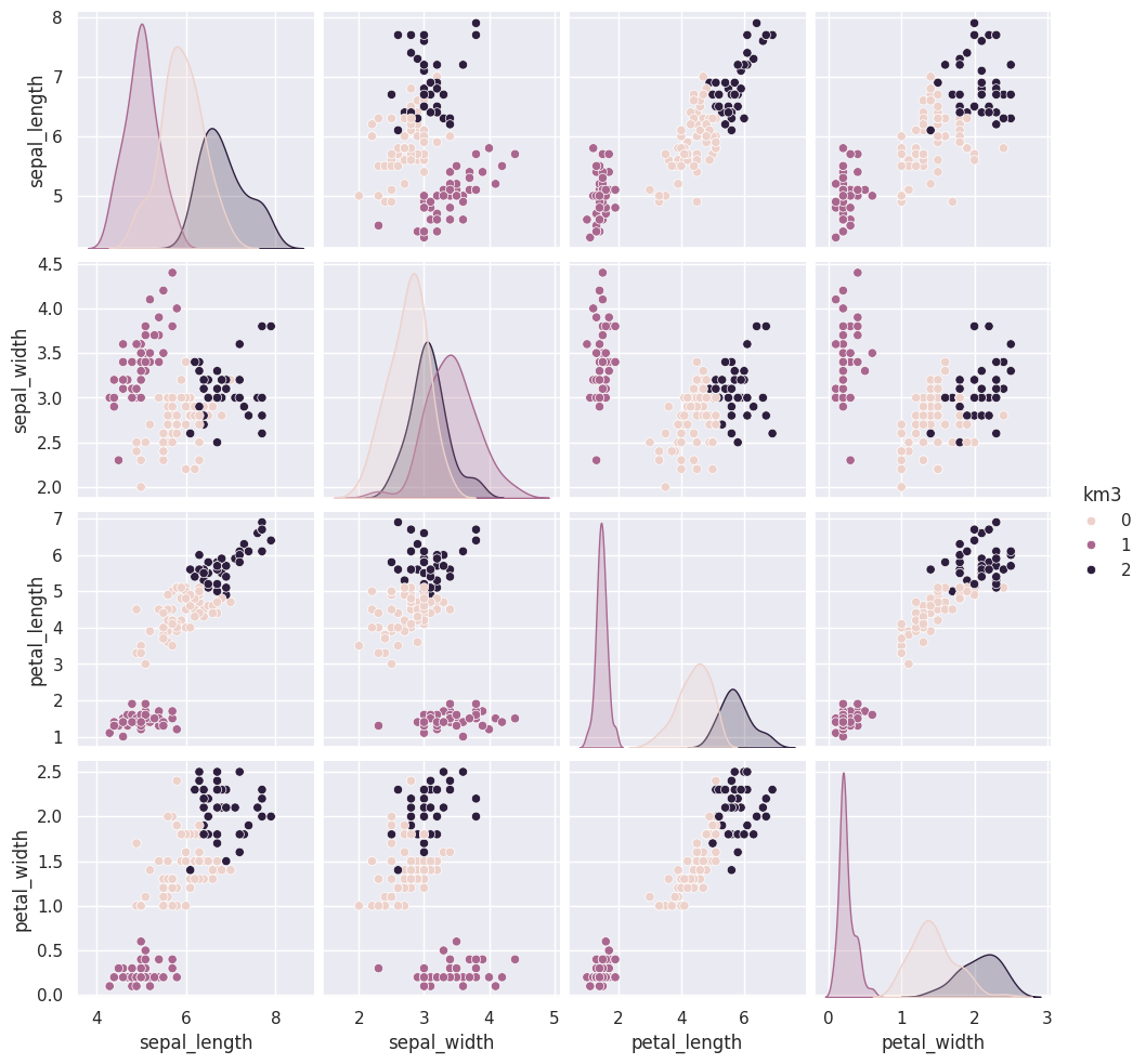
First we’ll save it in the dataframe
iris_df['km3'] = km.fit_predict(iris_X)
/opt/hostedtoolcache/Python/3.8.18/x64/lib/python3.8/site-packages/sklearn/cluster/_kmeans.py:1416: FutureWarning: The default value of `n_init` will change from 10 to 'auto' in 1.4. Set the value of `n_init` explicitly to suppress the warning
  super()._check_params_vs_input(X, default_n_init=10)
sns.pairplot(data=iris_df,hue='km3')
<seaborn.axisgrid.PairGrid at 0x7f6e01d86dc0>
For one pair of features we can look in more detail:
sns.relplot(data=iris_df,x = 'petal_width',y='sepal_width',
                hue='km3',style='species')
<seaborn.axisgrid.FacetGrid at 0x7f6df6e8a0d0>
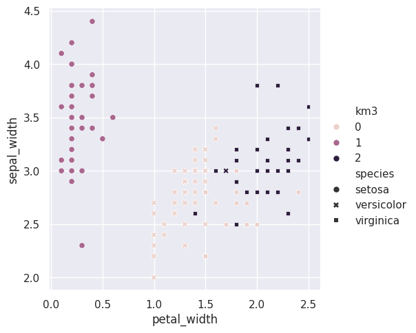
here i used the style to set the shape and the hue to set th color of the markers
so that we can see where the ground truth and learned groups agree and disagree.
14.4. Clustering Evaluation#
a: The mean distance between a sample and all other points in the same class.
b: The mean distance between a sample and all other points in the next nearest cluster.
This score computes a ratio of how close points are to points in the same cluster vs other clusters
In class, we drew pictures in prismia, but we can also generate samples to make a plot that shows a bad silhouette score:
Show code cell source
N = 100
# sample data that is one blob, in 2dimensions
bad_cluster_data = np.random.multivariate_normal([5,5],.75*np.eye(2), size=N)
data_cols = ['x0','x1']
df = pd.DataFrame(data=bad_cluster_data,columns=data_cols)
# randomly assign cluster labels with equal 50-50 probabilty for each sample
df['cluster'] = np.random.choice([0,1],N)

sns.relplot(data=df,x='x0',y='x1',hue='cluster',)
plt.title('S = ' + str(metrics.silhouette_score(df[data_cols],df['cluster'])));
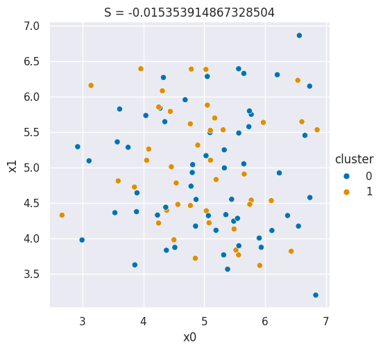
Here, since I generated the samples from one cluster and then assigned the cluster labels independently, randomly, for each point with no regard for its position the clustering score is pretty close to 0.
If, instead, I make more intentional clusters, we can see a better score:
And we can make a plot for a good silhouette score
Show code cell source
N = 50
# this is how far apart the points are within each cluster
#  (related to a)
spread = .05
# thisis how far apart the clusters are (realted to b)
distance = 50
# sample one cluster
single_cluster = np.random.multivariate_normal([1,1],
                                                spread*np.eye(2),
                                                 size=N)
#  make 2 copies, with a constant distance between them
good_cluster_data = np.concatenate([single_cluster,distance+single_cluster])
data_cols = ['x0','x1']
df = pd.DataFrame(data=good_cluster_data,columns=data_cols)
# label the points, since they're in order
df['cluster'] = [0]*N + [1]*N

sns.relplot(data=df,x='x0',y='x1',hue='cluster',)
plt.title('S = ' + str(metrics.silhouette_score(df[data_cols],df['cluster'])));
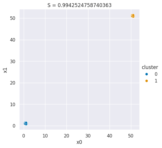
If you change the distance in the code above running it you can increase or decrase the score value
Then we can use the silhouette score on our existing clustering solution.
metrics.silhouette_score(iris_X,iris_df['km3'])
0.5528190123564102
We can also compare different numbers of clusters, we noted that in class it looked like maybe 2 might be better than 3, so lets look at that:
km2 = KMeans(n_clusters=2)
iris_df['km2'] = km2.fit_predict(iris_X)
metrics.silhouette_score(iris_X,iris_df['km2'])
/opt/hostedtoolcache/Python/3.8.18/x64/lib/python3.8/site-packages/sklearn/cluster/_kmeans.py:1416: FutureWarning: The default value of `n_init` will change from 10 to 'auto' in 1.4. Set the value of `n_init` explicitly to suppress the warning
  super()._check_params_vs_input(X, default_n_init=10)
0.6810461692117465
it is higher, as expected
we can also check 4:
km4 = KMeans(n_clusters=4)
iris_df['km4'] = km4.fit_predict(iris_X)
metrics.silhouette_score(iris_X,iris_df['km4'])
/opt/hostedtoolcache/Python/3.8.18/x64/lib/python3.8/site-packages/sklearn/cluster/_kmeans.py:1416: FutureWarning: The default value of `n_init` will change from 10 to 'auto' in 1.4. Set the value of `n_init` explicitly to suppress the warning
  super()._check_params_vs_input(X, default_n_init=10)
0.49805050499728815
it is not better, we can check more:
km10 = KMeans(n_clusters=10)
iris_df['km10'] = km10.fit_predict(iris_X)
metrics.silhouette_score(iris_X,iris_df['km10'])
/opt/hostedtoolcache/Python/3.8.18/x64/lib/python3.8/site-packages/sklearn/cluster/_kmeans.py:1416: FutureWarning: The default value of `n_init` will change from 10 to 'auto' in 1.4. Set the value of `n_init` explicitly to suppress the warning
  super()._check_params_vs_input(X, default_n_init=10)
0.32802357624839684
also not, so we would say that 2 clusters best describes this data.
14.5. Questions after class#
14.5.1. Is the pairplot slices of a 3d plot?#
Sort of, it’s actually 2D slcies of a 4D plot for the iris data because it has 4 features. We can think of the features like dimensions.
14.5.2. Why does the silhouette score not give a score for each predicted group? SInce the km3 columns in metrics.silhouette_score(iris_X, iris_df[‘km3’]) is the predicted categories, why is the silhouette score not separated for each km3?#
There is not an equivalent of confusion matrix in this concept, but we can get a score per sample and groupby to create a per group average:
iris_df['km3_silhouette'] = metrics.silhouette_samples(iris_X,iris_df['km3'])
iris_df.groupby('km3')['km3_silhouette'].mean()
km3
0    0.417320
1    0.798140
2    0.451105
Name: km3_silhouette, dtype: float64