18. Task Review and Cross Validation

18.1. ML Tasks

We learned classification first, because it shares similarities with each regression and clustering, while regression and clustering have less in common.

• Classification is supervised learning for a categorical target.

• Regression is supervised learning for a continuous target.

• Clustering is unsupervised learning for a categorical target.

We have used a small flowchart for the tasks:

flowchart TD labels{Do you have labels <br>in the dataset? } labels --> |yes| sup[Supervised Learning] labels --> |no| unsup[Unsupervised Learning] sup --> ltype{What type of variable <br> are the labels?} ltype --> |continuous| reg[Regression] ltype --> |discrete| clas[Classification] unsup --> groups{Do you think there are <br> groups within the data?} groups --> |yes | clus[Clutering]

Sklearn provides a nice flow chart for thinking through both tasks (big blocks) and models (the small green boxes)

Predicting a category is another way of saying categorical target. Predicting a quantitiy is another way of saying continuous target. Having lables or not is the difference between

The flowchart assumes you know what you want to do with data and that is the ideal scenario. You have a dataset and you have a goal. For the purpose of getting to practice with a variety of things, in this course we ask you to start with a task and then find a dataset. Assignment 9 is the last time that’s true however. Starting with Assignment 10, you can choose and focus on a specific application domain and then choose the right task from there.

Thinking about this, however, you use this information to move between the tasks within a given type of data. For example, you can use the same data for clustering as you did for classification. Switching the task changes the questions though: classification evaluation tells us how separable the classes are given that classifiers decision rule. Clustering can find other subgroups or the same ones, so the evaluation we choose allows us to explore this in more ways.

Regression requires a continuous target, so we need a dataset to be suitable for that, we can’t transform from the classification dataset to a regression one.
However, we can go the other way and that’s how some classification datasets are created.

The UCI adult Dataset is a popular ML dataset that was dervied from census data. The goal is to use a variety of features to predict if a person makes more than \(50k per year or not. While income is a continuous value, they applied a threshold (\)50k) to it to make a binary variable. The dataset does not include income in dollars, only the binary indicator.

Recent work reconstructed the dataset with the continuous valued income. Their repository contains the data as well as links to their paper and a video of their talk on it.

18.2. Cross Validation

This week our goal is to learn how to optmize models. The first step in that is to get a good estimate of its performance.

We have seen that the test train splits, which are random, influence the performance.

In order to find the best hyperparameters for the model on a given dataset, we need some better evaluation techniques.

# basic libraries
import numpy as np
import pandas as pd
import seaborn as sns
import matplotlib.pyplot as plt
# models classes
from sklearn import tree
from sklearn import cluster
from sklearn import svm
# datasets
from sklearn import datasets
# model selection tools
from sklearn.model_selection import GridSearchCV
from sklearn.model_selection import cross_val_score
from sklearn.model_selection import train_test_split
from sklearn.model_selection import KFold, ShuffleSplit
from sklearn import metrics

This week and next week together are about model selection or choosing what model we might want to actually use

18.2.1. Loading Data with sklearn

Note

in class we tried to use as_frame=True alone, but I had misread. To figure it out, I looked at the source code to see what it does, I saw that it does not return the structure for that case, but it does call it. This is also in the git blame view where I could see it had not changed recently. What it does is change the type of those attributes in the bunch or the two items returned if in the return_X_y, so here.

It does say that but is an easy thing to misinterpret. This is the advantage of open source code though, worst case, even if the documentation confuses you, you can see the actual code and see it.

This way we can get dataFrames:

iris_X, iris_y = datasets.load_iris(return_X_y=True,as_frame=True)
type(iris_X)

pandas.core.frame.DataFrame

or in the bunch

iris_bunch_frame= datasets.load_iris(as_frame=True)
type(iris_bunch.data)

---------------------------------------------------------------------------
NameError                                 Traceback (most recent call last)
Cell In[3], line 2
      1 iris_bunch_frame= datasets.load_iris(as_frame=True)
----> 2 type(iris_bunch.data)

NameError: name 'iris_bunch' is not defined

otherwise the bunch contains numpy arrays.

iris_bunch= datasets.load_iris()
type(iris_bunch.data)

numpy.ndarray

18.2.2. K-fold Cross Validation

We’ll use the Iris data with a decision tree.

We are going to use it this way for claass:

iris_X, iris_y = datasets.load_iris(return_X_y=True)

and instantiate a Decision tree see classificaiton notes about dt

dt = tree.DecisionTreeClassifier()

We can split the data, fit the model, then compute a score, but since the splitting is a randomized step, the score is a random variable.

For example, if we have a coin that we want to see if it’s fair or not. We would flip it to test. One flip doesn’t tell us, but if we flip it a few times, we can estimate the probability it is heads by counting how many of the flips are heads and dividing by how many flips.

We can do something similar with our model performance. We can split the data a bunch of times and compute the score each time.

cross_val_score does this all for us.

It takes an estimator object and the data.

By default it uses 5-fold cross validation. It splits the data into 5 sections, then uses 4 of them to train and one to test. It then iterates through so that each section gets used for testing.

cross_val_score(dt, iris_X, iris_y)

array([0.96666667, 0.96666667, 0.9       , 1.        , 1.        ])

We get back a score for each section or “fold” of the data. We can average those to get a single estimate.

To actually report, we would take the mean

Note

this is not the mean of the numbers from the cell above, because when we call the function again, it does another round of random splits

np.mean(cross_val_score(dt, iris_X, iris_y))

0.9600000000000002

We can change from 5-fold to 10-fold by setting the cv parameter

cross_val_score(dt, iris_X, iris_y,cv=10)

array([1.        , 0.93333333, 1.        , 0.93333333, 0.93333333,
       0.86666667, 0.93333333, 1.        , 1.        , 1.        ])

In K-fold cross validation, we split the data in K sections and train on K-1 and test one 1 section. So the percentages are like:

# K is the cv
K = 10
train_pct =(K-1)/K
test_pct = 1/K
train_pct, test_pct

(0.9, 0.1)

18.3. Cross validation is model-agnostic

We can use any estimator object here.

For example, we can apply it to clustering too:

km = cluster.KMeans(n_clusters = 3)

cross_val_score(km, iris_X)

/opt/hostedtoolcache/Python/3.8.18/x64/lib/python3.8/site-packages/sklearn/cluster/_kmeans.py:1416: FutureWarning: The default value of `n_init` will change from 10 to 'auto' in 1.4. Set the value of `n_init` explicitly to suppress the warning
  super()._check_params_vs_input(X, default_n_init=10)
/opt/hostedtoolcache/Python/3.8.18/x64/lib/python3.8/site-packages/sklearn/cluster/_kmeans.py:1416: FutureWarning: The default value of `n_init` will change from 10 to 'auto' in 1.4. Set the value of `n_init` explicitly to suppress the warning
  super()._check_params_vs_input(X, default_n_init=10)
/opt/hostedtoolcache/Python/3.8.18/x64/lib/python3.8/site-packages/sklearn/cluster/_kmeans.py:1416: FutureWarning: The default value of `n_init` will change from 10 to 'auto' in 1.4. Set the value of `n_init` explicitly to suppress the warning
  super()._check_params_vs_input(X, default_n_init=10)
/opt/hostedtoolcache/Python/3.8.18/x64/lib/python3.8/site-packages/sklearn/cluster/_kmeans.py:1416: FutureWarning: The default value of `n_init` will change from 10 to 'auto' in 1.4. Set the value of `n_init` explicitly to suppress the warning
  super()._check_params_vs_input(X, default_n_init=10)
/opt/hostedtoolcache/Python/3.8.18/x64/lib/python3.8/site-packages/sklearn/cluster/_kmeans.py:1416: FutureWarning: The default value of `n_init` will change from 10 to 'auto' in 1.4. Set the value of `n_init` explicitly to suppress the warning
  super()._check_params_vs_input(X, default_n_init=10)

array([ -9.062     , -14.93195873, -18.93234207, -23.70894258,
       -19.55457726])

18.4. Details and types of Cross validation

First, lets look at the Kfold cross validation object. Under the hood, this is the default thing that cross_val_score uses 1

Cross validation objects are all examples of the splitter type in sklearn

we can instantiate one of these too:

kf = KFold(n_splits=10)

it returns the splits as a generator

Note

Generators return an item each time you call it in a list, instead of building the whole list up front, which makes it more memory efficient.

the Python wiki has a good generator example and the official docs have a more technical description

splits = kf.split(iris_X, iris_y)
splits

<generator object _BaseKFold.split at 0x7f808f9b99e0>

jupyter does not know how to display it, so it jsut says the type.

type(splits)

generator

type(range(3))

range

We can use this in a loop to get the list of indices that will be used to get the test and train data for each fold. To visualize what this is doing, see below.

Warning

I changed this to create an empty list and append a dataframe to it each time through the list then create a combined dataframe after to remove the

N_samples = len(iris_y)
kf_tt_list = []
i = 1
for train_idx, test_idx in splits:
    
    # make a list of "unused"
    col_data =  np.asarray(['unused']*N_samples)
    # fill in train and test by the indices
    col_data[train_idx] = 'Train'
    col_data[test_idx] = 'Test'
    kf_tt_list.append(pd.DataFrame(data = col_data,index=list(range(N_samples)), columns = ['split ' + str(i)]))
    i +=1

kf_tt_df = pd.concat(kf_tt_list,axis=1)

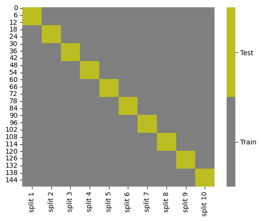
Note that unlike test_train_split this does not always randomize and shuffle the data before splitting.

kf_tt_df

	split 1	split 2	split 3	split 4	split 5	split 6	split 7	split 8	split 9	split 10
0	Test	Train	Train	Train	Train	Train	Train	Train	Train	Train
1	Test	Train	Train	Train	Train	Train	Train	Train	Train	Train
2	Test	Train	Train	Train	Train	Train	Train	Train	Train	Train
3	Test	Train	Train	Train	Train	Train	Train	Train	Train	Train
4	Test	Train	Train	Train	Train	Train	Train	Train	Train	Train
...	...	...	...	...	...	...	...	...	...	...
145	Train	Train	Train	Train	Train	Train	Train	Train	Train	Test
146	Train	Train	Train	Train	Train	Train	Train	Train	Train	Test
147	Train	Train	Train	Train	Train	Train	Train	Train	Train	Test
148	Train	Train	Train	Train	Train	Train	Train	Train	Train	Test
149	Train	Train	Train	Train	Train	Train	Train	Train	Train	Test

150 rows × 10 columns

We can also visualize:

cmap = sns.color_palette("tab10",10)
g = sns.heatmap(kf_tt_df.replace({'Test':1,'Train':0}),cmap=cmap[7:9],cbar_kws={'ticks':[.25,.75]},linewidths=0,
    linecolor='gray')
colorbar = g.collections[0].colorbar
colorbar.set_ticklabels(['Train','Test'])

We can also see another splitter(this is what train_test_split uses)

skf = ShuffleSplit(10)
N_samples = len(iris_y)
ss_tt_list = []
i = 1
for train_idx, test_idx in skf.split(iris_X, iris_y):
    col_data = np.asarray(['unused']*N_samples)
    col_data[train_idx] = 'Train'
    col_data[test_idx] = 'Test'
    ss_tt_list.append(pd.DataFrame(data = col_data, index=list(range(N_samples))), columns=['split' + str(i)])
    i +=1

ss_tt_df = pd.concat(ss_tt_list,axis=1)
ss_tt_df

---------------------------------------------------------------------------
TypeError                                 Traceback (most recent call last)
Cell In[20], line 9
      7     col_data[train_idx] = 'Train'
      8     col_data[test_idx] = 'Test'
----> 9     ss_tt_list.append(pd.DataFrame(data = col_data, index=list(range(N_samples))), columns=['split' + str(i)])
     10     i +=1
     12 ss_tt_df = pd.concat(ss_tt_list,axis=1)

TypeError: append() takes no keyword arguments

cmap = sns.color_palette("tab10",10)
g = sns.heatmap(ss_tt_df.replace({'Test':1,'Train':0}),cmap=cmap[7:9],cbar_kws={'ticks':[.25,.75]},linewidths=0,
    linecolor='gray')
colorbar = g.collections[0].colorbar
colorbar.set_ticklabels(['Train','Test'])

---------------------------------------------------------------------------
NameError                                 Traceback (most recent call last)
Cell In[21], line 2
      1 cmap = sns.color_palette("tab10",10)
----> 2 g = sns.heatmap(ss_tt_df.replace({'Test':1,'Train':0}),cmap=cmap[7:9],cbar_kws={'ticks':[.25,.75]},linewidths=0,
      3     linecolor='gray')
      4 colorbar = g.collections[0].colorbar
      5 colorbar.set_ticklabels(['Train','Test'])

NameError: name 'ss_tt_df' is not defined

we can see this is different and more random.

We can also use it in cross_val_score

cross_val_score(dt,iris_X,iris_y,cv=ShuffleSplit(n_splits=100,test_size=.2))

array([0.96666667, 0.96666667, 0.93333333, 1.        , 0.93333333,
       1.        , 0.96666667, 0.86666667, 1.        , 0.96666667,
       0.86666667, 0.96666667, 0.96666667, 1.        , 0.93333333,
       0.93333333, 0.93333333, 0.9       , 0.9       , 0.96666667,
       0.93333333, 0.93333333, 0.93333333, 0.93333333, 0.93333333,
       1.        , 0.93333333, 0.96666667, 1.        , 0.96666667,
       0.96666667, 0.96666667, 0.93333333, 0.96666667, 0.96666667,
       0.93333333, 1.        , 0.96666667, 1.        , 0.96666667,
       0.96666667, 1.        , 0.9       , 0.96666667, 0.93333333,
       1.        , 0.96666667, 0.93333333, 0.96666667, 0.93333333,
       1.        , 0.9       , 0.96666667, 1.        , 0.93333333,
       1.        , 0.96666667, 1.        , 0.96666667, 0.96666667,
       0.96666667, 0.93333333, 0.93333333, 1.        , 0.96666667,
       0.93333333, 0.96666667, 0.96666667, 0.9       , 1.        ,
       0.96666667, 0.93333333, 0.93333333, 0.96666667, 0.93333333,
       0.96666667, 0.96666667, 0.9       , 0.96666667, 0.9       ,
       1.        , 0.86666667, 0.9       , 0.9       , 0.96666667,
       0.93333333, 0.9       , 0.96666667, 0.96666667, 0.96666667,
       1.        , 0.96666667, 0.96666667, 0.9       , 0.93333333,
       0.96666667, 0.96666667, 0.93333333, 0.9       , 0.96666667])

18.5. Questions after class

18.5.1. When should you change test and train sizes rather than just using the default?

Having more training data often gets you a better model, having more test samples gives you a better idea of how well the model will work on new data. You have to make that choice.

I think sometimes trying a few and seeing if the performance changes much or not, can also help you decide, if it doesn’t matter much, then use the default. If it changes a lot, then maybe use as much data as possible for training and you can go as far as KFold cross validation with K = len(X) which is called leave-one-out cross validation.

---

1

actually above, since we used a classifier it actually used stratified cross validaiton whichh solves the problem we discussed in class where the data as sorted and that could be misleading. StratifiedKfold makes each fold (section) have the same percentage of each class for the classifier. It only does this if the estimator is a classifier, for clustering and regression it always does regular Kfold.