
13. Classification Models#
First machine learning model: Naive bayes
import pandas as pd
import seaborn as sns
from sklearn import tree
import numpy as np
from sklearn.model_selection import train_test_split
from sklearn.naive_bayes import GaussianNB
from sklearn.metrics import confusion_matrix, classification_report, roc_auc_score
import matplotlib.pyplot as plt

iris_df = sns.load_dataset('iris')
To start we will look at the data
iris_df.head()
| sepal_length | sepal_width | petal_length | petal_width | species | |
|---|---|---|---|---|---|
| 0 | 5.1 | 3.5 | 1.4 | 0.2 | setosa |
| 1 | 4.9 | 3.0 | 1.4 | 0.2 | setosa |
| 2 | 4.7 | 3.2 | 1.3 | 0.2 | setosa |
| 3 | 4.6 | 3.1 | 1.5 | 0.2 | setosa |
| 4 | 5.0 | 3.6 | 1.4 | 0.2 | setosa |
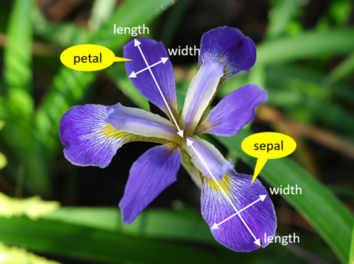
We’re trying to build an automatic flower classifier that, for measurements of a new flower returns the predicted species. To do this, we have a DataFrame with columns for species, petal width, petal length, sepal length, and sepal width. The species is what type of flower it is the petal and sepal are parts of the flower.
Show code cell content
iris_df.columns
Index(['sepal_length', 'sepal_width', 'petal_length', 'petal_width',
       'species'],
      dtype='object')
The species will be the target and the measurements will be the features. We want to predict the target from the features, the species from the measurements.
feature_vars = ['sepal_length', 'sepal_width', 'petal_length', 'petal_width']
target_var = 'species'
13.1. What does Naive Bayes do?#
Naive = indepdent features
Bayes = most probable
More resources:
We can look at this data using a pair plot. It plots each pair of numerical variables in a grid of scatterplots and on the diagonal (where it would be a variable with itself) shows the distribution of that variable.
sns.pairplot(data =iris_df,hue=target_var)
<seaborn.axisgrid.PairGrid at 0x7fa27b99b6a0>
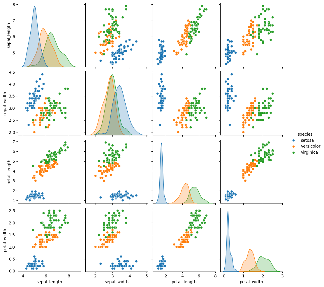
This data is reasonably separable beacuse the different species (indicated with colors in the plot) do not overlap much. We see that the features are distributed sort of like a normal, or Gaussian, distribution. In 2D a Gaussian distribution is like a hill, so we expect to see more points near the center and fewer on the edge of circle-ish blobs. These blobs are slightly live ovals, but not too skew.
This means that the assumptions of the Gaussian Naive Bayes model are met well enough we can expect the classifier to do well.
13.2. Separating Training and Test Data#
To do machine learning, we split the data both sample wise (rows if tidy) and variable-wise (columns if tidy). First, we’ll designate the columns to use as features and as the target.
The features are the input that we wish to use to predict the target.
Next, we’ll use a sklearn function to split the data randomly into test and train portions.
X_train, X_test, y_train, y_test = train_test_split(iris_df[feature_vars],
                                                    iris_df[target_var],
                                                    random_state=5)
This function returns multiple values, the docs say that it returns twice as many as it is passed. We passed two separate things, the features and the labels separated, so we get train and test each for both.
Note
If you get different numbers for the index than I do here or run the train test split multipe times and see things change, you have a different ranomd seed above.
X_train.head()
| sepal_length | sepal_width | petal_length | petal_width | |
|---|---|---|---|---|
| 40 | 5.0 | 3.5 | 1.3 | 0.3 |
| 115 | 6.4 | 3.2 | 5.3 | 2.3 |
| 142 | 5.8 | 2.7 | 5.1 | 1.9 |
| 69 | 5.6 | 2.5 | 3.9 | 1.1 |
| 17 | 5.1 | 3.5 | 1.4 | 0.3 |
X_train.shape, X_test.shape
((112, 4), (38, 4))
We can see by default how many samples it puts the training set:
len(X_train)/len(iris_df)
0.7466666666666667
So by default we get a 75-25 split.
13.3. Instantiating our Model Object#
Next we will instantiate the object for our model. In sklearn they call these objects estimator. All estimators have a similar usage. First we instantiate the object and set any hyperparameters.
Instantiating the object says we are assuming a particular type of model. In this case Gaussian Naive Bayes. This sets several assumptions in one form:
we assume data are Gaussian (normally) distributed
the features are uncorrelated/independent (Naive)
the best way to predict is to find the highest probability (Bayes)
this is one example of a Bayes Estimator
gnb = GaussianNB()
At this point the object is not very interesting
gnb.__dict__
{'priors': None, 'var_smoothing': 1e-09}
The fit method uses the data to learn the model’s parameters. In this case, a Gaussian distribution is characterized by a mean and variance; so the GNB classifier is characterized by one mean and one variance for each class (in 4d, like our data)
gnb.fit(X_train,y_train)
GaussianNB()In a Jupyter environment, please rerun this cell to show the HTML representation or trust the notebook.
On GitHub, the HTML representation is unable to render, please try loading this page with nbviewer.org.
GaussianNB()
The attributes of the estimator object (gbn) describe the data (eg the class list) and the model’s parameters. The theta_ (often in math as \(\theta\) or \(\mu\))
represents the mean and the var_ (\(\sigma\)) represents the variance of the
distributions.
gnb.__dict__
{'priors': None,
 'var_smoothing': 1e-09,
 'classes_': array(['setosa', 'versicolor', 'virginica'], dtype='<U10'),
 'feature_names_in_': array(['sepal_length', 'sepal_width', 'petal_length', 'petal_width'],
       dtype=object),
 'n_features_in_': 4,
 'epsilon_': 3.1373206313775512e-09,
 'theta_': array([[5.00526316, 3.45263158, 1.45      , 0.23421053],
        [5.96666667, 2.75277778, 4.26666667, 1.31944444],
        [6.55789474, 2.98684211, 5.52105263, 2.02631579]]),
 'var_': array([[0.14207757, 0.16196676, 0.03460527, 0.00698754],
        [0.26611111, 0.10471451, 0.21722223, 0.03767747],
        [0.40770083, 0.1090374 , 0.32745153, 0.06193906]]),
 'class_count_': array([38., 36., 38.]),
 'class_prior_': array([0.33928571, 0.32142857, 0.33928571])}
13.3.1. Scoring a model#
Estimator objects also have a score method. If the estimator is a classifier, that score is accuracy. We will see that for other types of estimators it is different types.
gnb.score(X_test,y_test)
0.9210526315789473
13.4. Making model predictions#
we can predict for each sample as well:
y_pred = gnb.predict(X_test)
Important
in the end of class I tried to demo this and got an error
We can also do one single sample, the iloc attrbiute lets us pick out rows by
integer index even if that is not the actual index of the DataFrame
X_test.iloc[0]
sepal_length    5.8
sepal_width     2.7
petal_length    3.9
petal_width     1.2
Name: 82, dtype: float64
but if we pick one row, it returns a series, which is incompatible with the predict method.
gnb.predict(X_test.iloc[0])
/opt/hostedtoolcache/Python/3.8.18/x64/lib/python3.8/site-packages/sklearn/base.py:465: UserWarning: X does not have valid feature names, but GaussianNB was fitted with feature names
  warnings.warn(
---------------------------------------------------------------------------
ValueError                                Traceback (most recent call last)
Cell In[17], line 1
----> 1 gnb.predict(X_test.iloc[0])

File /opt/hostedtoolcache/Python/3.8.18/x64/lib/python3.8/site-packages/sklearn/naive_bayes.py:101, in _BaseNB.predict(self, X)
     87 """
     88 Perform classification on an array of test vectors X.
     89
   (...)
     98     Predicted target values for X.
     99 """
    100 check_is_fitted(self)
--> 101 X = self._check_X(X)
    102 jll = self._joint_log_likelihood(X)
    103 return self.classes_[np.argmax(jll, axis=1)]

File /opt/hostedtoolcache/Python/3.8.18/x64/lib/python3.8/site-packages/sklearn/naive_bayes.py:269, in GaussianNB._check_X(self, X)
    267 def _check_X(self, X):
    268     """Validate X, used only in predict* methods."""
--> 269     return self._validate_data(X, reset=False)

File /opt/hostedtoolcache/Python/3.8.18/x64/lib/python3.8/site-packages/sklearn/base.py:605, in BaseEstimator._validate_data(self, X, y, reset, validate_separately, cast_to_ndarray, **check_params)
    603         out = X, y
    604 elif not no_val_X and no_val_y:
--> 605     out = check_array(X, input_name="X", **check_params)
    606 elif no_val_X and not no_val_y:
    607     out = _check_y(y, **check_params)

File /opt/hostedtoolcache/Python/3.8.18/x64/lib/python3.8/site-packages/sklearn/utils/validation.py:938, in check_array(array, accept_sparse, accept_large_sparse, dtype, order, copy, force_all_finite, ensure_2d, allow_nd, ensure_min_samples, ensure_min_features, estimator, input_name)
    936     # If input is 1D raise error
    937     if array.ndim == 1:
--> 938         raise ValueError(
    939             "Expected 2D array, got 1D array instead:\narray={}.\n"
    940             "Reshape your data either using array.reshape(-1, 1) if "
    941             "your data has a single feature or array.reshape(1, -1) "
    942             "if it contains a single sample.".format(array)
    943         )
    945 if dtype_numeric and hasattr(array.dtype, "kind") and array.dtype.kind in "USV":
    946     raise ValueError(
    947         "dtype='numeric' is not compatible with arrays of bytes/strings."
    948         "Convert your data to numeric values explicitly instead."
    949     )

ValueError: Expected 2D array, got 1D array instead:
array=[5.8 2.7 3.9 1.2].
Reshape your data either using array.reshape(-1, 1) if your data has a single feature or array.reshape(1, -1) if it contains a single sample.
If we select with a range, that only includes 1, it still returns a DataFrame
X_test.iloc[0:1]
| sepal_length | sepal_width | petal_length | petal_width | |
|---|---|---|---|---|
| 82 | 5.8 | 2.7 | 3.9 | 1.2 |
which we can get a prediction for:
gnb.predict(X_test.iloc[0:1])
array(['versicolor'], dtype='<U10')
We could also transform with to_frame and then transpose with T or (transpose)
gnb.predict(X_test.iloc[0].to_frame().T)
array(['versicolor'], dtype='<U10')
We can also pass a 2D array (list of lists) with values in it (here I typed in values similar to the mean for setosa above)
gnb.predict([[5.1, 3.6, 1.5, 0.25]])
/opt/hostedtoolcache/Python/3.8.18/x64/lib/python3.8/site-packages/sklearn/base.py:465: UserWarning: X does not have valid feature names, but GaussianNB was fitted with feature names
  warnings.warn(
array(['setosa'], dtype='<U10')
This way it warns us that the feature names are missing, but it still gives a prediction.
13.4.1. Evaluating Performance in more detail#
confusion_matrix(y_test,y_pred)
array([[12,  0,  0],
       [ 0, 13,  1],
       [ 0,  2, 10]])
This is a little harder to read than the 2D version but we can make it a dataframe to read it better.
n_classes = len(gnb.classes_)
prediction_labels = [['predicted class']*n_classes, gnb.classes_]
actual_labels = [['true class']*n_classes, gnb.classes_]
conf_mat = confusion_matrix(y_test,y_pred)
conf_df = pd.DataFrame(data = conf_mat, index=actual_labels, columns=prediction_labels)
Show code cell content
from myst_nb import glue
c1 = gnb.classes_[1]
c2 = gnb.classes_[2]
conf12 = conf_mat[1][2]
glue('c1',c1)
glue('c2',c2)
glue('f1t2',conf12)
'versicolor'
'virginica'
1
1 flowers were mistakenly classified as ‘versicolor’ when they were really ‘virginica’
This report is also available:
print(classification_report(y_test,y_pred))
              precision    recall  f1-score   support

      setosa       1.00      1.00      1.00        12
  versicolor       0.87      0.93      0.90        14
   virginica       0.91      0.83      0.87        12

    accuracy                           0.92        38
   macro avg       0.93      0.92      0.92        38
weighted avg       0.92      0.92      0.92        38
We can also get a report with a few metrics.
Recall is the percent of each species that were predicted correctly.
Precision is the percent of the ones predicted to be in a species that are truly that species.
the F1 score is combination of the two
We see we have perfect recall and precision for setosa, as above, but we have lower for the other two because there were mistakes where versicolor and virginica were mixed up.
13.5. What does a generative model mean?#
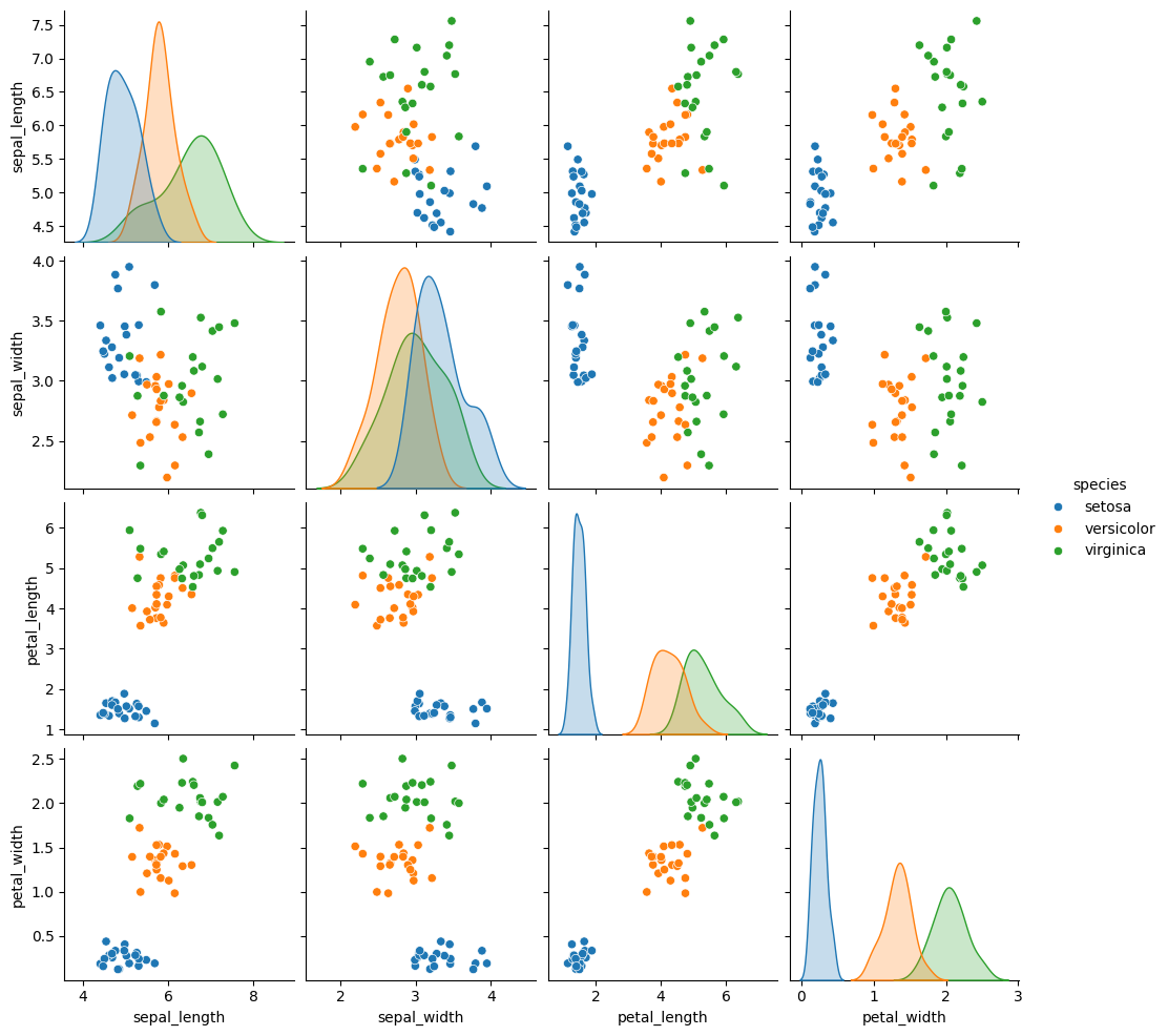
Gaussian Naive Bayes is a very simple model, but it is a generative model (in constrast to a discriminative model) so we can use it to generate synthetic data that looks like the real data, based on what the model learned.
N = 20
n_features = len(feature_vars)
gnb_df = pd.DataFrame(np.concatenate([np.random.multivariate_normal(th, sig*np.eye(n_features),N)
                 for th, sig in zip(gnb.theta_,gnb.var_)]),
                 columns = gnb.feature_names_in_)
gnb_df['species'] = [ci for cl in [[c]*N for c in gnb.classes_] for ci in cl]
sns.pairplot(data =gnb_df, hue='species')
<seaborn.axisgrid.PairGrid at 0x7fa275d44dc0>
To break this code down:
To do this, we extract the mean and variance parameters from the model
(gnb.theta_,gnb.sigma_) and zip them together to create an iterable object
that in each iteration returns one value from each list (for th, sig in zip(gnb.theta_,gnb.sigma_)).
We do this inside of a list comprehension and for each th,sig where th is
from gnb.theta_ and sig is from gnb.sigma_ we use np.random.multivariate_normal
to get 20 samples. In a general multivariate normal distribution the second parameter is actually a covariance
matrix. This describes both the variance of each individual feature and the
correlation of the features. Since Naive Bayes is Naive it assumes the features
are independent or have 0 correlation. So, to create the matrix from the vector
of variances we multiply by np.eye(4) which is the identity matrix or a matrix
with 1 on the diagonal and 0 elsewhere. Finally we stack the groups for each
species together with np.concatenate (like pd.concat but works on numpy objects
and np.random.multivariate_normal returns numpy arrays not data frames) and put all of that in a
DataFrame using the feature names as the columns.
Then we add a species column, by repeating each species 20 times
[c]*N for c in gnb.classes_ and then unpack that into a single list instead of
as list of lists.
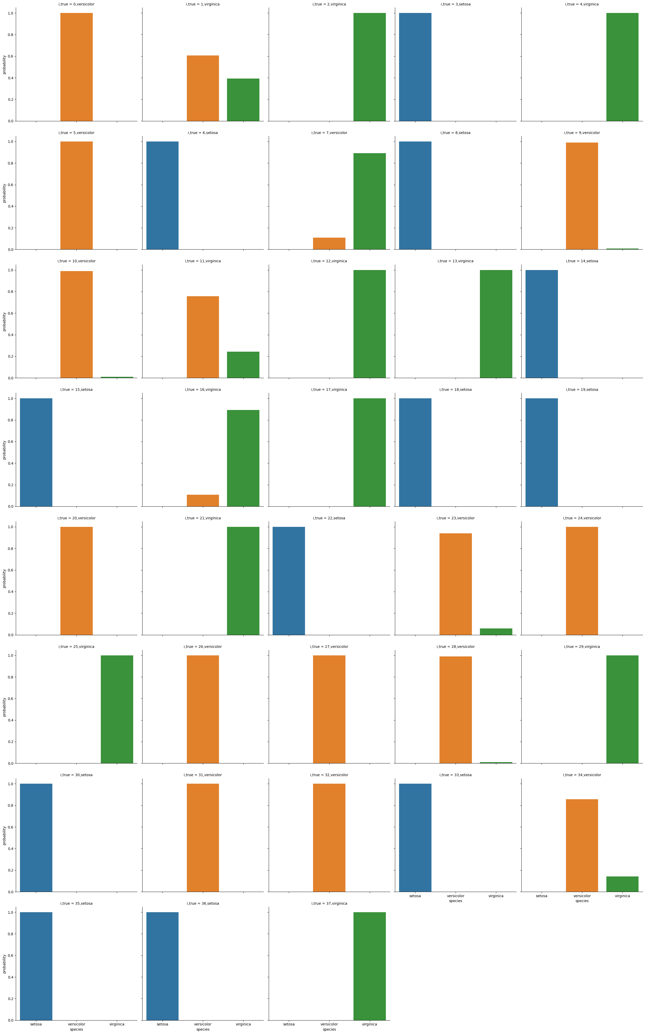
13.6. How does it make the predictions?#
It computes the probability for each class and then predicts the highest one:
gnb.predict_proba(X_test)
array([[4.98983163e-068, 9.99976886e-001, 2.31140535e-005],
       [2.38605399e-151, 6.05788555e-001, 3.94211445e-001],
       [1.52930285e-229, 6.40965644e-007, 9.99999359e-001],
       [1.00000000e+000, 3.59116140e-019, 4.35301434e-027],
       [2.95380506e-300, 1.34947916e-012, 1.00000000e+000],
       [2.16647395e-038, 9.99999791e-001, 2.08857492e-007],
       [1.00000000e+000, 1.05055556e-017, 6.59080633e-026],
       [9.55629438e-147, 1.08807974e-001, 8.91192026e-001],
       [1.00000000e+000, 2.52482409e-016, 1.46364748e-024],
       [6.02158895e-108, 9.90558853e-001, 9.44114652e-003],
       [2.10951969e-108, 9.88848490e-001, 1.11515105e-002],
       [1.45542701e-135, 7.56061808e-001, 2.43938192e-001],
       [8.96514127e-239, 1.55965373e-007, 9.99999844e-001],
       [5.55336438e-231, 1.60582831e-006, 9.99998394e-001],
       [1.00000000e+000, 3.60824506e-014, 6.21633393e-022],
       [1.00000000e+000, 1.29808311e-010, 2.24314344e-018],
       [3.09565382e-153, 1.07603601e-001, 8.92396399e-001],
       [3.81317125e-230, 1.03976329e-006, 9.99998960e-001],
       [1.00000000e+000, 1.37507763e-015, 5.26100959e-023],
       [1.00000000e+000, 1.15359632e-018, 7.80287600e-027],
       [2.60921281e-078, 9.99821175e-001, 1.78824945e-004],
       [2.59248282e-219, 8.60114059e-006, 9.99991399e-001],
       [1.00000000e+000, 2.18609042e-018, 7.77596623e-026],
       [2.27597506e-127, 9.40305572e-001, 5.96944278e-002],
       [8.22137518e-080, 9.99794097e-001, 2.05903463e-004],
       [1.19322368e-231, 1.64825193e-007, 9.99999835e-001],
       [2.39789249e-089, 9.98853183e-001, 1.14681677e-003],
       [1.09087833e-083, 9.99736540e-001, 2.63460309e-004],
       [2.25963865e-110, 9.88633468e-001, 1.13665324e-002],
       [3.92002893e-231, 1.15859357e-006, 9.99998841e-001],
       [1.00000000e+000, 7.65551108e-018, 1.19398607e-025],
       [1.76892853e-077, 9.99969673e-001, 3.03269074e-005],
       [6.37930105e-045, 9.99999177e-001, 8.23423901e-007],
       [1.00000000e+000, 3.51305986e-018, 1.33290716e-025],
       [3.91957440e-113, 8.57857810e-001, 1.42142190e-001],
       [1.00000000e+000, 2.70877085e-018, 3.42709168e-026],
       [9.99999997e-001, 2.88681309e-009, 1.12890422e-016],
       [4.10240137e-278, 9.44646226e-011, 1.00000000e+000]])
we can also plot these
# make the probabilities into a dataframe labeled with classes & make the index a separate column
prob_df = pd.DataFrame(data = gnb.predict_proba(X_test), columns = gnb.classes_ ).reset_index()
# add the predictions
prob_df['predicted_species'] = y_pred
prob_df['true_species'] = y_test.values
# for plotting, make a column that combines the index & prediction
pred_text = lambda r: str( r['index']) + ',' + r['predicted_species']
prob_df['i,pred'] = prob_df.apply(pred_text,axis=1)
# same for ground truth
true_text = lambda r: str( r['index']) + ',' + r['true_species']
prob_df['correct'] = prob_df['predicted_species'] == prob_df['true_species']
# a dd a column for which are correct
prob_df['i,true'] = prob_df.apply(true_text,axis=1)
prob_df_melted = prob_df.melt(id_vars =[ 'index', 'predicted_species','true_species','i,pred','i,true','correct'],value_vars = gnb.classes_,
                             var_name = target_var, value_name = 'probability')
prob_df_melted.head()
| index | predicted_species | true_species | i,pred | i,true | correct | species | probability | |
|---|---|---|---|---|---|---|---|---|
| 0 | 0 | versicolor | versicolor | 0,versicolor | 0,versicolor | True | setosa | 4.989832e-68 |
| 1 | 1 | versicolor | virginica | 1,versicolor | 1,virginica | False | setosa | 2.386054e-151 |
| 2 | 2 | virginica | virginica | 2,virginica | 2,virginica | True | setosa | 1.529303e-229 |
| 3 | 3 | setosa | setosa | 3,setosa | 3,setosa | True | setosa | 1.000000e+00 |
| 4 | 4 | virginica | virginica | 4,virginica | 4,virginica | True | setosa | 2.953805e-300 |
and then we can plot this:
# plot a bar graph for each point labeled with the prediction
sns.catplot(data =prob_df_melted, x = 'species', y='probability' ,col ='i,true',
            col_wrap=5,kind='bar', hue='species')
<seaborn.axisgrid.FacetGrid at 0x7fa27454eca0>
13.7. What if the assumptions are not met?#
Using a toy dataset here shows an easy to see challenge for the classifier that we have seen so far. Real datasets will be hard in different ways, and since they’re higher dimensional, it’s harder to visualize the cause.
corner_data = 'https://raw.githubusercontent.com/rhodyprog4ds/06-naive-bayes/f425ba121cc0c4dd8bcaa7ebb2ff0b40b0b03bff/data/dataset6.csv'
df6= pd.read_csv(corner_data,usecols=[1,2,3])
sns.pairplot(data=df6, hue='char',hue_order=['A','B'])
<seaborn.axisgrid.PairGrid at 0x7fa26b10cfa0>
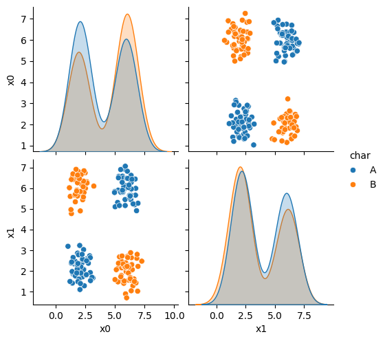
As we can see in this dataset, these classes are quite separated.
X_train, X_test, y_train, y_test = train_test_split(df6[['x0','x1']],
                          df6['char'],
                          random_state = 4)
gnb_corners = GaussianNB()
gnb_corners.fit(X_train,y_train)
gnb_corners.score(X_test, y_test)
0.72
But we do not get a very good classification score.
To see why, we can look at what it learned.
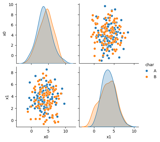
N = 100
gnb_df = pd.DataFrame(np.concatenate([np.random.multivariate_normal(th, sig*np.eye(2),N)
         for th, sig in zip(gnb_corners.theta_,gnb_corners.var_)]),
         columns = ['x0','x1'])
gnb_df['char'] = [ci for cl in [[c]*N for c in gnb_corners.classes_] for ci in cl]

sns.pairplot(data =gnb_df, hue='char',hue_order=['A','B'])
<seaborn.axisgrid.PairGrid at 0x7fa26849fb50>
df6_pred = X_test.copy()
df6_pred['pred'] = gnb_corners.predict(X_test)
sns.pairplot(data =df6_pred, hue ='pred', hue_order =['A','B'])
<seaborn.axisgrid.PairGrid at 0x7fa268286160>
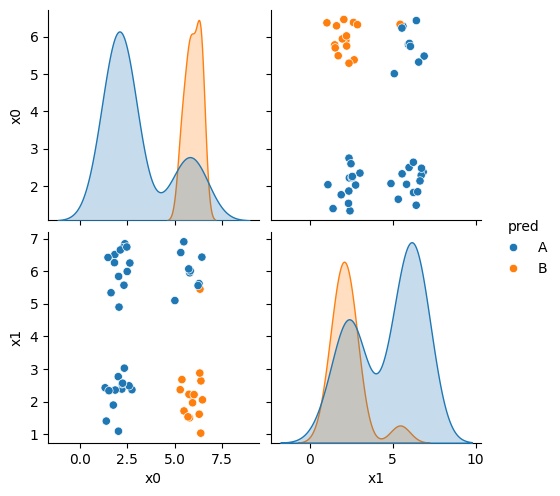
This does not look much like the data and it’s hard to tell which is higher at any given point in the 2D space. We know though, that it has missed the mark. We can also look at the actual predictions.
If you try this again, split, fit, plot, it will learn different decisions, but always at least about 25% of the data will have to be classified incorrectly.
13.8. Decision Trees#
This data does not fit the assumptions of the Niave Bayes model, but a decision tree has a different rule. It can be more complex, but for the scikit learn one relies on splitting the data at a series of points along one feature at a time, sequentially. It basically learns a flowchart for deciding what class the sample belongs to at test time
It is a discriminative model, because it describes how to discriminate (in the sense of differentiate) between the classes. This is in contrast to the generative model that describes how the data is distributed.
That said, sklearn makes using new classifiers really easy once have learned one. All of the classifiers have the same API (same methods and attributes).
dt = tree.DecisionTreeClassifier()
dt.fit(X_train,y_train)
dt.score(X_test,y_test)
1.0
The sklearn estimator objects (that corresond to different models) all have the same API, so the fit, predict, and score methods are the same as above. We will see this also in regression and clustering. What each method does in terms of the specific calculations will vary depending on the model, but they’re always there.
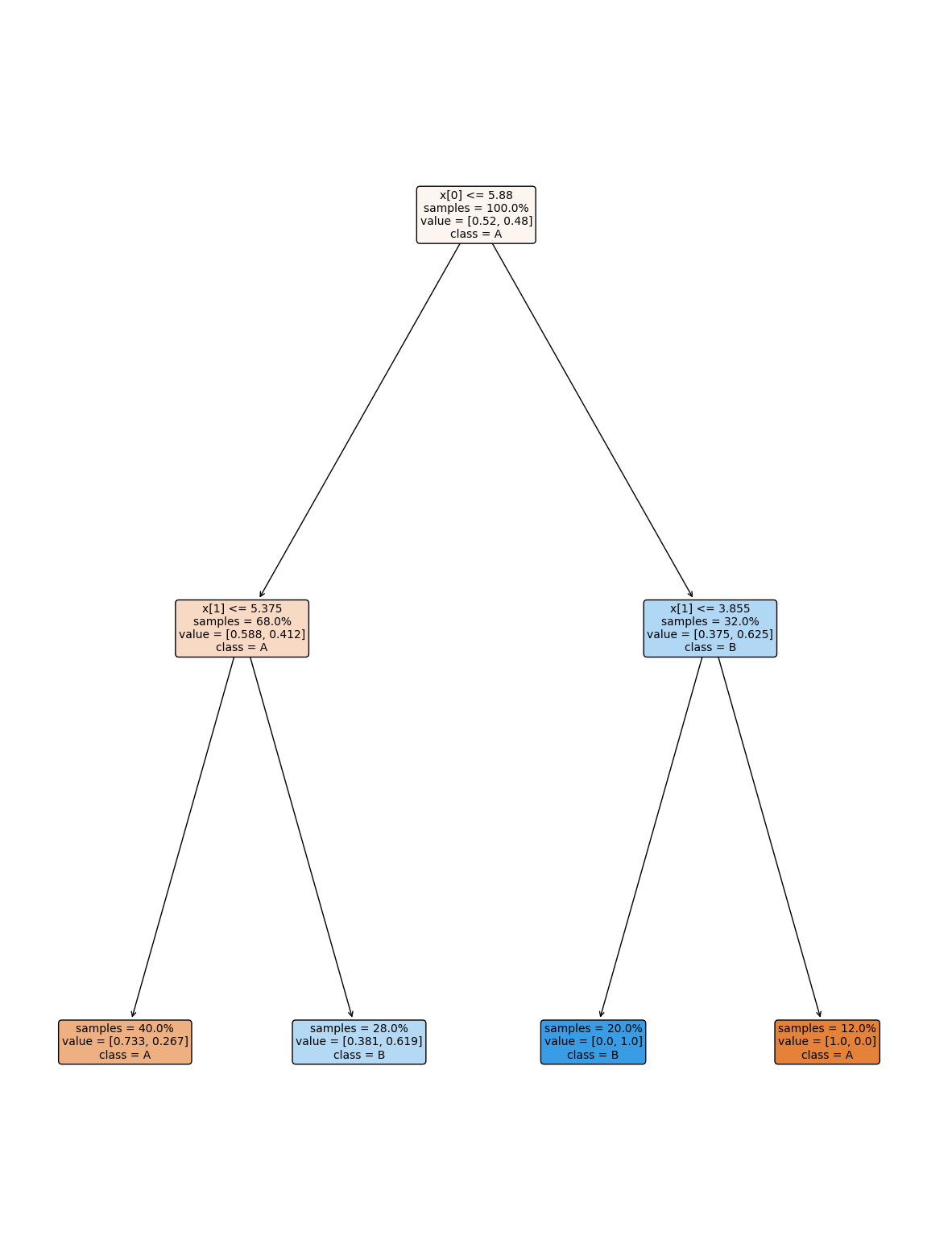
the tree module also allows you to plot the tree to examine it.
plt.figure(figsize=(15,20))
tree.plot_tree(dt, rounded =True, class_names = ['A','B'],
      proportion=True, filled =True, impurity=False,fontsize=10);

On the iris dataset, the sklearn docs include a diagram showing the decision boundary You should be able to modify this for another classifier.
13.9. Setting Classifier Parameters#
The decision tree we had above has a lot more layers than we would expect. This is really simple data so we still got perfect classification. However, the more complex the model, the more risk that it will learn something noisy about the training data that doesn’t hold up in the test set.
Fortunately, we can control the parameters to make it find a simpler decision boundary.
dt2 = tree.DecisionTreeClassifier(max_depth=2)
dt2.fit(X_train,y_train)
dt2.score(X_test,y_test)
0.74
plt.figure(figsize=(15,20))
tree.plot_tree(dt2, rounded =True, class_names = ['A','B'],
      proportion=True, filled =True, impurity=False,fontsize=10);
13.10. Questions#
Note
I added in some questions from previous semesters because few questions were asked.
13.10.1. Are there any good introductions to ScikitLearn that you are aware of?#
Scikit Learn User Guide is the best one and they have a large example gallery.
13.10.2. Are there any popular machine learning models that use decision trees?#
Yes, a lot of medical appilcations do, because since they are easy to understand, it is easier for healthcare providers to trust them.
13.10.3. Do predictive algorithms have pros and cons? Or is there a standard?#
Each algorithm has different properties and strengths and weaknesses. Some are more popular than others, but they all do have weaknesses.
13.10.4. how often should we use confusion matrixes? Would it be better just to check the accuracy without one?#
A confusion matrix gives more detail on the performance than accuracy alone. If the accuracy was like 99.99 maybe the confustion matrix is not informative, but otherwise, it is generally useful to understand what types of mistakes as context for how you might use/not use/ trust the model.
13.10.5. Due to the initial ‘shuffling’ of data: Is it possible to get a seed/shuffle of data split so that it that does much worse in a model?#
Yes you can get a bad split, we will see next week a statistical technique that helps us improve this. However, the larger your dataset, the less likely this will happen, so we mostly now just get bigger and bigger datasets.
13.10.6. How does gnb = GaussianNB() work?#
this line calls the GaussianNB class constructor method with all default paramters.
This means it creates and object of that type, we can see that like follows
gnb_ex = GaussianNB()
type(gnb_ex)
sklearn.naive_bayes.GaussianNB
13.10.7. how will level 3s work?#
I will update on level 3s in class on Tuesday (and the site before then)
13.10.8. Could we use strata to better identify the the data in the toy dataset?#
The dataset didn’t have any additional columns we could use to stratify this data, this data
is simply not a good fit for GaussianNB because it does not fit the assumptions.
Above I included the Decision Tree example, so you can see a classifer that does work for it.
13.10.9. is it possible after training the model to add more data to it ?#
The models we will see in class, no. However, there is a thing called “online learning” that involves getting more data on a regular basis to improve its performance.
13.10.10. Can you use machine learning for any type of data?#
Yes the features for example could be an image instead of four numbers. It could also be text. The basic ideas are the same for more complex data, so we are going to spend a lot of time building your understanding of what ML is on simple data. Past students have successfully applied ML in more complex data after this course because once you have a good understanding of the core ideas, applying it to other forms of data is easier to learn on your own.
13.10.11. Can we check how well the model did using the y_test df?#
we could compare them directly or using score that does.
y_pred == y_test
/tmp/ipykernel_2076/1082399451.py:1: FutureWarning: elementwise comparison failed; returning scalar instead, but in the future will perform elementwise comparison
  y_pred == y_test
---------------------------------------------------------------------------
ValueError                                Traceback (most recent call last)
Cell In[41], line 1
----> 1 y_pred == y_test

File /opt/hostedtoolcache/Python/3.8.18/x64/lib/python3.8/site-packages/pandas/core/ops/common.py:81, in _unpack_zerodim_and_defer.<locals>.new_method(self, other)
     77             return NotImplemented
     79 other = item_from_zerodim(other)
---> 81 return method(self, other)

File /opt/hostedtoolcache/Python/3.8.18/x64/lib/python3.8/site-packages/pandas/core/arraylike.py:40, in OpsMixin.__eq__(self, other)
     38 @unpack_zerodim_and_defer("__eq__")
     39 def __eq__(self, other):
---> 40     return self._cmp_method(other, operator.eq)

File /opt/hostedtoolcache/Python/3.8.18/x64/lib/python3.8/site-packages/pandas/core/series.py:6096, in Series._cmp_method(self, other, op)
   6093 rvalues = extract_array(other, extract_numpy=True, extract_range=True)
   6095 with np.errstate(all="ignore"):
-> 6096     res_values = ops.comparison_op(lvalues, rvalues, op)
   6098 return self._construct_result(res_values, name=res_name)

File /opt/hostedtoolcache/Python/3.8.18/x64/lib/python3.8/site-packages/pandas/core/ops/array_ops.py:270, in comparison_op(left, right, op)
    265 if isinstance(rvalues, (np.ndarray, ABCExtensionArray)):
    266     # TODO: make this treatment consistent across ops and classes.
    267     #  We are not catching all listlikes here (e.g. frozenset, tuple)
    268     #  The ambiguous case is object-dtype.  See GH#27803
    269     if len(lvalues) != len(rvalues):
--> 270         raise ValueError(
    271             "Lengths must match to compare", lvalues.shape, rvalues.shape
    272         )
    274 if should_extension_dispatch(lvalues, rvalues) or (
    275     (isinstance(rvalues, (Timedelta, BaseOffset, Timestamp)) or right is NaT)
    276     and not is_object_dtype(lvalues.dtype)
    277 ):
    278     # Call the method on lvalues
    279     res_values = op(lvalues, rvalues)

ValueError: ('Lengths must match to compare', (50,), (38,))
sum(y_pred == y_test)/len(y_test)
/tmp/ipykernel_2076/369106620.py:1: FutureWarning: elementwise comparison failed; returning scalar instead, but in the future will perform elementwise comparison
  sum(y_pred == y_test)/len(y_test)
---------------------------------------------------------------------------
ValueError                                Traceback (most recent call last)
Cell In[42], line 1
----> 1 sum(y_pred == y_test)/len(y_test)

File /opt/hostedtoolcache/Python/3.8.18/x64/lib/python3.8/site-packages/pandas/core/ops/common.py:81, in _unpack_zerodim_and_defer.<locals>.new_method(self, other)
     77             return NotImplemented
     79 other = item_from_zerodim(other)
---> 81 return method(self, other)

File /opt/hostedtoolcache/Python/3.8.18/x64/lib/python3.8/site-packages/pandas/core/arraylike.py:40, in OpsMixin.__eq__(self, other)
     38 @unpack_zerodim_and_defer("__eq__")
     39 def __eq__(self, other):
---> 40     return self._cmp_method(other, operator.eq)

File /opt/hostedtoolcache/Python/3.8.18/x64/lib/python3.8/site-packages/pandas/core/series.py:6096, in Series._cmp_method(self, other, op)
   6093 rvalues = extract_array(other, extract_numpy=True, extract_range=True)
   6095 with np.errstate(all="ignore"):
-> 6096     res_values = ops.comparison_op(lvalues, rvalues, op)
   6098 return self._construct_result(res_values, name=res_name)

File /opt/hostedtoolcache/Python/3.8.18/x64/lib/python3.8/site-packages/pandas/core/ops/array_ops.py:270, in comparison_op(left, right, op)
    265 if isinstance(rvalues, (np.ndarray, ABCExtensionArray)):
    266     # TODO: make this treatment consistent across ops and classes.
    267     #  We are not catching all listlikes here (e.g. frozenset, tuple)
    268     #  The ambiguous case is object-dtype.  See GH#27803
    269     if len(lvalues) != len(rvalues):
--> 270         raise ValueError(
    271             "Lengths must match to compare", lvalues.shape, rvalues.shape
    272         )
    274 if should_extension_dispatch(lvalues, rvalues) or (
    275     (isinstance(rvalues, (Timedelta, BaseOffset, Timestamp)) or right is NaT)
    276     and not is_object_dtype(lvalues.dtype)
    277 ):
    278     # Call the method on lvalues
    279     res_values = op(lvalues, rvalues)

ValueError: ('Lengths must match to compare', (50,), (38,))
gnb.score(X_test,y_test)
---------------------------------------------------------------------------
ValueError                                Traceback (most recent call last)
Cell In[43], line 1
----> 1 gnb.score(X_test,y_test)

File /opt/hostedtoolcache/Python/3.8.18/x64/lib/python3.8/site-packages/sklearn/base.py:706, in ClassifierMixin.score(self, X, y, sample_weight)
    681 """
    682 Return the mean accuracy on the given test data and labels.
    683
   (...)
    702     Mean accuracy of ``self.predict(X)`` w.r.t. `y`.
    703 """
    704 from .metrics import accuracy_score
--> 706 return accuracy_score(y, self.predict(X), sample_weight=sample_weight)

File /opt/hostedtoolcache/Python/3.8.18/x64/lib/python3.8/site-packages/sklearn/naive_bayes.py:101, in _BaseNB.predict(self, X)
     87 """
     88 Perform classification on an array of test vectors X.
     89
   (...)
     98     Predicted target values for X.
     99 """
    100 check_is_fitted(self)
--> 101 X = self._check_X(X)
    102 jll = self._joint_log_likelihood(X)
    103 return self.classes_[np.argmax(jll, axis=1)]

File /opt/hostedtoolcache/Python/3.8.18/x64/lib/python3.8/site-packages/sklearn/naive_bayes.py:269, in GaussianNB._check_X(self, X)
    267 def _check_X(self, X):
    268     """Validate X, used only in predict* methods."""
--> 269     return self._validate_data(X, reset=False)

File /opt/hostedtoolcache/Python/3.8.18/x64/lib/python3.8/site-packages/sklearn/base.py:580, in BaseEstimator._validate_data(self, X, y, reset, validate_separately, cast_to_ndarray, **check_params)
    509 def _validate_data(
    510     self,
    511     X="no_validation",
   (...)
    516     **check_params,
    517 ):
    518     """Validate input data and set or check the `n_features_in_` attribute.
    519
    520     Parameters
   (...)
    578         validated.
    579     """
--> 580     self._check_feature_names(X, reset=reset)
    582     if y is None and self._get_tags()["requires_y"]:
    583         raise ValueError(
    584             f"This {self.__class__.__name__} estimator "
    585             "requires y to be passed, but the target y is None."
    586         )

File /opt/hostedtoolcache/Python/3.8.18/x64/lib/python3.8/site-packages/sklearn/base.py:507, in BaseEstimator._check_feature_names(self, X, reset)
    502 if not missing_names and not unexpected_names:
    503     message += (
    504         "Feature names must be in the same order as they were in fit.\n"
    505     )
--> 507 raise ValueError(message)

ValueError: The feature names should match those that were passed during fit.
Feature names unseen at fit time:
- x0
- x1
Feature names seen at fit time, yet now missing:
- petal_length
- petal_width
- sepal_length
- sepal_width
We can also use any of the other metrics we saw, we’ll practice more on Wednesday
13.10.12. I want to know more about the the test_train_split() function#
the docs are a good place to start.