4. Exploratory Data Analysis

Now we get to start actual data science!

4.1. First, a note on assignments

4.1.1. the goal

• I am not looking for “an answer”

• You should not be either

• I am looking for evidence that you understand the material (thus far including prereqs)

• You should be trying to understand material

This means that in office hours, I am going to:

• ask you questions to help you think about the problem and the material

• help direct your attention to the right part of the error message to figure out what is wrong

4.1.2. Getting help

Sending me a screenshot is almost guaranteed to not get you a help. Not because I do not want to, but because I literally do not have the information to get you an answer.

Typically when someone do not know how to fix something from the error message, it is because they are reading the wrong part of the error message or looking at the wrong part of the code trying to find the problem.

This means they end up screenshotting that wrong thing, so I literally cannot tell what is wrong from the screenshot.

I am not being stubborn, I just literally cannot tell what is wrong because I do not have enough information. Debugging code requires context, if you deprive me that, then I cannot help.

To get asynchronous help:

• upload your whole notebook, errors and all

• create an issue on that repo

4.2. This week: Exploratory Data Analysis

• How to summarize data

• Interpretting summaries

• Visualizing data

• interpretting summaries

4.2.1. Summarizing and Visualizing Data are very important

• People cannot interpret high dimensional or large samples quickly

• Important in EDA to help you make decisions about the rest of your analysis

• Important in how you report your results

• Summaries are similar calculations to performance metrics we will see later

• visualizations are often essential in debugging models

THEREFORE

• You have a lot of chances to earn summarize and visualize

• we will be picky when we assess if you earned them or not

import pandas as pd

coffee_data_url = 'https://raw.githubusercontent.com/jldbc/coffee-quality-database/master/data/robusta_data_cleaned.csv'
coffee_df = pd.read_csv(coffee_data_url, index_col=0)

coffee_df.head(1)

	Species	Owner	Country.of.Origin	Farm.Name	Lot.Number	Mill	ICO.Number	Company	Altitude	Region	...	Color	Category.Two.Defects	Expiration	Certification.Body	Certification.Address	Certification.Contact	unit_of_measurement	altitude_low_meters	altitude_high_meters	altitude_mean_meters
1	Robusta	ankole coffee producers coop	Uganda	kyangundu cooperative society	NaN	ankole coffee producers	0	ankole coffee producers coop	1488	sheema south western	...	Green	2	June 26th, 2015	Uganda Coffee Development Authority	e36d0270932c3b657e96b7b0278dfd85dc0fe743	03077a1c6bac60e6f514691634a7f6eb5c85aae8	m	1488.0	1488.0	1488.0

1 rows × 43 columns

4.3. Describing a Dataset

So far, we’ve loaded data in a few different ways and then we’ve examined DataFrames as a data structure, looking at what different attributes they have and what some of the methods are, and how to get data into them.

We can also get more structural information with the info

coffee_df.info()

<class 'pandas.core.frame.DataFrame'>
Index: 28 entries, 1 to 28
Data columns (total 43 columns):
 #   Column                 Non-Null Count  Dtype  
---  ------                 --------------  -----  
 0   Species                28 non-null     object 
 1   Owner                  28 non-null     object 
 2   Country.of.Origin      28 non-null     object 
 3   Farm.Name              25 non-null     object 
 4   Lot.Number             6 non-null      object 
 5   Mill                   20 non-null     object 
 6   ICO.Number             17 non-null     object 
 7   Company                28 non-null     object 
 8   Altitude               25 non-null     object 
 9   Region                 26 non-null     object 
 10  Producer               26 non-null     object 
 11  Number.of.Bags         28 non-null     int64  
 12  Bag.Weight             28 non-null     object 
 13  In.Country.Partner     28 non-null     object 
 14  Harvest.Year           28 non-null     int64  
 15  Grading.Date           28 non-null     object 
 16  Owner.1                28 non-null     object 
 17  Variety                3 non-null      object 
 18  Processing.Method      10 non-null     object 
 19  Fragrance...Aroma      28 non-null     float64
 20  Flavor                 28 non-null     float64
 21  Aftertaste             28 non-null     float64
 22  Salt...Acid            28 non-null     float64
 23  Bitter...Sweet         28 non-null     float64
 24  Mouthfeel              28 non-null     float64
 25  Uniform.Cup            28 non-null     float64
 26  Clean.Cup              28 non-null     float64
 27  Balance                28 non-null     float64
 28  Cupper.Points          28 non-null     float64
 29  Total.Cup.Points       28 non-null     float64
 30  Moisture               28 non-null     float64
 31  Category.One.Defects   28 non-null     int64  
 32  Quakers                28 non-null     int64  
 33  Color                  25 non-null     object 
 34  Category.Two.Defects   28 non-null     int64  
 35  Expiration             28 non-null     object 
 36  Certification.Body     28 non-null     object 
 37  Certification.Address  28 non-null     object 
 38  Certification.Contact  28 non-null     object 
 39  unit_of_measurement    28 non-null     object 
 40  altitude_low_meters    25 non-null     float64
 41  altitude_high_meters   25 non-null     float64
 42  altitude_mean_meters   25 non-null     float64
dtypes: float64(15), int64(5), object(23)
memory usage: 9.6+ KB

Now, we can actually start to analyze the data itself.

The describe method provides us with a set of summary statistics that broadly

coffee_df.describe()

	Number.of.Bags	Harvest.Year	Fragrance...Aroma	Flavor	Aftertaste	Salt...Acid	Bitter...Sweet	Mouthfeel	Uniform.Cup	Clean.Cup	Balance	Cupper.Points	Total.Cup.Points	Moisture	Category.One.Defects	Quakers	Category.Two.Defects	altitude_low_meters	altitude_high_meters	altitude_mean_meters
count	28.000000	28.000000	28.000000	28.000000	28.000000	28.000000	28.000000	28.000000	28.000000	28.000000	28.000000	28.000000	28.000000	28.000000	28.000000	28.0	28.000000	25.00000	25.000000	25.000000
mean	168.000000	2013.964286	7.702500	7.630714	7.559643	7.657143	7.675714	7.506786	9.904286	9.928214	7.541786	7.761429	80.868929	0.065714	2.964286	0.0	1.892857	1367.60000	1387.600000	1377.600000
std	143.226317	1.346660	0.296156	0.303656	0.342469	0.261773	0.317063	0.725152	0.238753	0.211030	0.526076	0.330507	2.441233	0.058464	12.357280	0.0	2.601129	838.06205	831.884207	833.980216
min	1.000000	2012.000000	6.750000	6.670000	6.500000	6.830000	6.670000	5.080000	9.330000	9.330000	5.250000	6.920000	73.750000	0.000000	0.000000	0.0	0.000000	40.00000	40.000000	40.000000
25%	1.000000	2013.000000	7.580000	7.560000	7.397500	7.560000	7.580000	7.500000	10.000000	10.000000	7.500000	7.580000	80.170000	0.000000	0.000000	0.0	0.000000	795.00000	795.000000	795.000000
50%	170.000000	2014.000000	7.670000	7.710000	7.670000	7.710000	7.750000	7.670000	10.000000	10.000000	7.670000	7.830000	81.500000	0.100000	0.000000	0.0	1.000000	1095.00000	1200.000000	1100.000000
75%	320.000000	2015.000000	7.920000	7.830000	7.770000	7.830000	7.830000	7.830000	10.000000	10.000000	7.830000	7.920000	82.520000	0.120000	0.000000	0.0	2.000000	1488.00000	1488.000000	1488.000000
max	320.000000	2017.000000	8.330000	8.080000	7.920000	8.000000	8.420000	8.250000	10.000000	10.000000	8.000000	8.580000	83.750000	0.130000	63.000000	0.0	9.000000	3170.00000	3170.000000	3170.000000

further reading

On the documentation page for describe the “ See Also” shows the links to the documentation of most of the individual functions. This is a good way to learn about other things, or find something when you are not quite sure what it would be named. Go to a function thats similar to what you want and then look at the related functions.

From this, we can draw several conclusions. FOr example straightforward ones like:

• the smallest number of bags rated is 1 and at least 25% of the coffees rates only had 1 bag

• the first ratings included were 2012 and last in 2017 (min & max)

• the mean Mouthfeel was 7.5

• Category One defects are not very common ( the 75th% is 0)

Or more nuanced ones that compare across variables like

• the raters scored coffee higher on Uniformity.Cup and Clean.Cup than other scores (mean score; only on the ones that seem to have a scale of up to 8/10)

• the coffee varied more in Mouthfeel and Balance that most other scores (the std; only on the ones that seem to have a scale of of up to 8/10)

• there are 3 ratings with no altitude (count of other variables is 28; alt is 25)

And these all give us a sense of the values and the distribution or spread fo the data in each column.

4.3.1. Understanding Quantiles

The 50% has another more common name: the median. It means 50% of the data are lower (and higher) than this value.

4.3.2. Individual variable

We can use the descriptive statistics on individual columns as well.

coffee_df['Balance'].descirbe()

---------------------------------------------------------------------------
AttributeError                            Traceback (most recent call last)
/tmp/ipykernel_2089/957071290.py in ?()
----> 1 coffee_df['Balance'].descirbe()

/opt/hostedtoolcache/Python/3.8.18/x64/lib/python3.8/site-packages/pandas/core/generic.py in ?(self, name)
   5985             and name not in self._accessors
   5986             and self._info_axis._can_hold_identifiers_and_holds_name(name)
   5987         ):
   5988             return self[name]
-> 5989         return object.__getattribute__(self, name)

AttributeError: 'Series' object has no attribute 'descirbe'

This is an AttributeError because there is no method or property of a pd.Series that is named 'descirbe' that tells me it is a typo.

coffee_df['Balance'].describe()

count    28.000000
mean      7.541786
std       0.526076
min       5.250000
25%       7.500000
50%       7.670000
75%       7.830000
max       8.000000
Name: Balance, dtype: float64

4.4. Individual statistics

We can also extract each of the statistics that the describe method calculates individually, by name.

coffee_df.mean(numeric_only=True)

Number.of.Bags           168.000000
Harvest.Year            2013.964286
Fragrance...Aroma          7.702500
Flavor                     7.630714
Aftertaste                 7.559643
Salt...Acid                7.657143
Bitter...Sweet             7.675714
Mouthfeel                  7.506786
Uniform.Cup                9.904286
Clean.Cup                  9.928214
Balance                    7.541786
Cupper.Points              7.761429
Total.Cup.Points          80.868929
Moisture                   0.065714
Category.One.Defects       2.964286
Quakers                    0.000000
Category.Two.Defects       1.892857
altitude_low_meters     1367.600000
altitude_high_meters    1387.600000
altitude_mean_meters    1377.600000
dtype: float64

coffee_df.min(numeric_only=True)

Number.of.Bags             1.00
Harvest.Year            2012.00
Fragrance...Aroma          6.75
Flavor                     6.67
Aftertaste                 6.50
Salt...Acid                6.83
Bitter...Sweet             6.67
Mouthfeel                  5.08
Uniform.Cup                9.33
Clean.Cup                  9.33
Balance                    5.25
Cupper.Points              6.92
Total.Cup.Points          73.75
Moisture                   0.00
Category.One.Defects       0.00
Quakers                    0.00
Category.Two.Defects       0.00
altitude_low_meters       40.00
altitude_high_meters      40.00
altitude_mean_meters      40.00
dtype: float64

The quantiles are tricky, we cannot just .25%() to get the 25% percentile, we have to use the quantile method and pass it a value between 0 and 1.

coffee_df['Flavor'].quantile(.8)

7.83

coffee_df['Aftertaste'].mean()

7.559642857142856

4.5. Working with categorical data

There are different columns in the describe than the the whole dataset:

coffee_df.columns

Index(['Species', 'Owner', 'Country.of.Origin', 'Farm.Name', 'Lot.Number',
       'Mill', 'ICO.Number', 'Company', 'Altitude', 'Region', 'Producer',
       'Number.of.Bags', 'Bag.Weight', 'In.Country.Partner', 'Harvest.Year',
       'Grading.Date', 'Owner.1', 'Variety', 'Processing.Method',
       'Fragrance...Aroma', 'Flavor', 'Aftertaste', 'Salt...Acid',
       'Bitter...Sweet', 'Mouthfeel', 'Uniform.Cup', 'Clean.Cup', 'Balance',
       'Cupper.Points', 'Total.Cup.Points', 'Moisture', 'Category.One.Defects',
       'Quakers', 'Color', 'Category.Two.Defects', 'Expiration',
       'Certification.Body', 'Certification.Address', 'Certification.Contact',
       'unit_of_measurement', 'altitude_low_meters', 'altitude_high_meters',
       'altitude_mean_meters'],
      dtype='object')

So far, the stats above are only for numerical features.

We can get the prevalence of each one with value_counts

coffee_df['Color'].value_counts()

Color
Green           20
Blue-Green       3
Bluish-Green     2
Name: count, dtype: int64

Try it Yourself

Note value_counts does not count the NaN values, but count counts all of the not missing values and the shape of the DataFrame is the total number of rows. How can you get the number of missing Colors?

Describe only operates on the numerical columns, but we might want to know about the others. We can get the number of each value with value_counts

What is the most common country of origin?

coffee_df['Country.of.Origin'].value_counts()

Country.of.Origin
India            13
Uganda           10
United States     2
Ecuador           2
Vietnam           1
Name: count, dtype: int64

Value counts returns a pandas Series that has two parts: values and index

coffee_df['Country.of.Origin'].value_counts().values

array([13, 10,  2,  2,  1])

coffee_df['Country.of.Origin'].value_counts().index

Index(['India', 'Uganda', 'United States', 'Ecuador', 'Vietnam'], dtype='object', name='Country.of.Origin')

The max method takes the max of the values.

coffee_df['Country.of.Origin'].value_counts().max()

13

We can get the name of the most common country out of this Series using idmax

coffee_df['Country.of.Origin'].value_counts().idxmax()

'India'

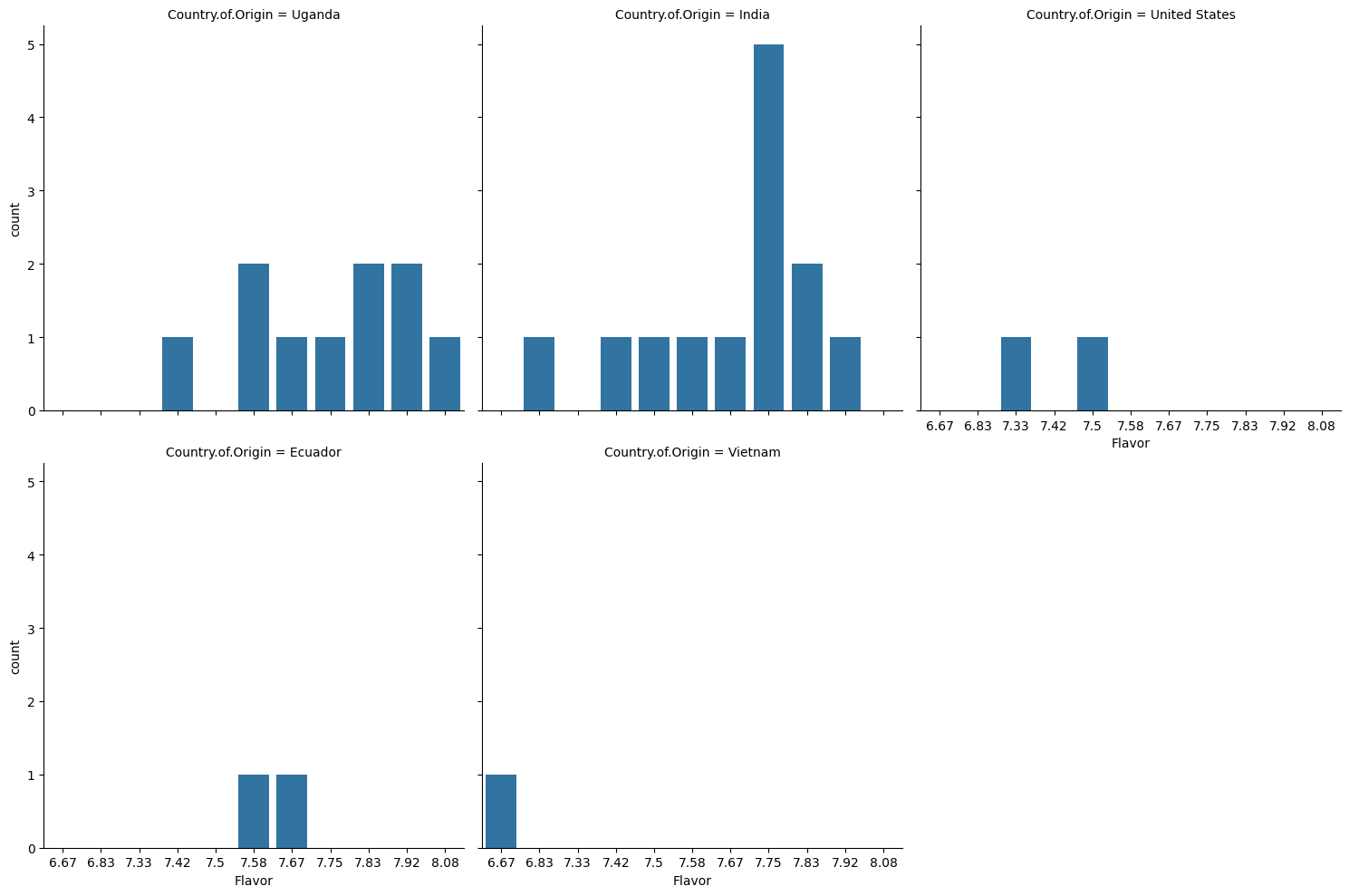
4.6. Which country scores highest on flavor?

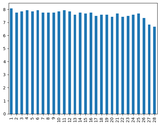
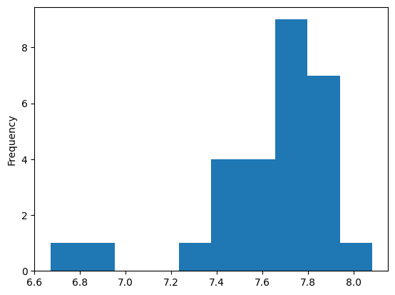
Let’s try to answer this with plots first

coffee_df['Flavor'].plot(kind='bar')

<Axes: >

coffee_df['Flavor'].plot(kind='hist')

<Axes: ylabel='Frequency'>

Seaborn give us opinionated defaults

import seaborn as sns

seaborn’s alias is sns as an inside joke among the developers to the character, Samual Norman Seaborn from West Wing they named the library after per their FAQ

So we can choose a typoe of plot and give it the whole dataframe and pass the variables to different parameters for them to be used in different ways.

sns.catplot(data =coffee_df, x='Flavor',kind ='count',col='Country.of.Origin',
           col_wrap=3)

<seaborn.axisgrid.FacetGrid at 0x7fce587e5e20>

4.6.1. Are any coffees more than one standard deviation above the average in Flavor ?

coffee_df['Flavor'].mean() + coffee_df['Flavor'].std(), coffee_df['Flavor'].max()

(7.93437014076549, 8.08)

Yes, one is more than one standard deviation from the mean.

4.7. Questions after class

4.7.1. can pycharm access urls?

Probably, it should not block them and they are language features, but I do not use it to know.

4.7.2. can we do what we did today in pycharm?

In theory, but pycharm probably will not handle the plots gracefully.

For this class, you need to submit notebook files, so pycharm will not work.

Pycharm is not typically used in datascience.

4.7.3. Are the bars on the Seaborn plot random colors, or do the colors have some meaning?

here, each different value is a different color. We wil control it more on Thursday

4.7.4. what types of jobs use what we learned today

Any data science role would use these skills daily.

4.7.5. Is there an equivalent for the index of the minimum value, such as idxmin()?

4.7.6. What is the std

standard deviation pandas docs on calculation. The wikipedia article on standard deviation is a good source on this.

4.7.7. Why can we not use matplotlib?

You can and you may for some customizaiton, but seaborn usually makes things faster to code and easier to read. I will not teach much matplotlib, but if you know it, up to date, not outdated, you may use it in some cases.

4.7.8. One question I have is what exactly the series object can be used for

A series is one column or one row of a dataframe.

4.7.9. how these lines of code can be used more efficiently in larger data sets?

For extremely large datasets if it’s too much to plot, you might, for exaple, sample the dataset to only plot a subset.

Otherwise this will still work.

4.7.10. Can you change what the plot graphs rather than an index vs frequency?

yes, we can change the plot to whatever we want.

4.7.11. actually I would like to know like with our country/flavor example can they be put in the same plot but with different colors for the different countries to each country side by side for a given score

yes

4.7.12. Can assignment 3 can be release so we can pre-read it over.

Yes, it is posted now

4.8. Questions we’ll answer in class on thurday

Important

These are great questions, I’m just not going to answer them here and then again in class on Thursday

• What other types of graphs could be used?

• Is there a way to use both x and y in sns without creating multiple charts?

• Using matplotlib, we never got to use it to class, and I want to know the difference between that and seanborn

• How to change the colors of the plots.

• What do we usually tend to look for in terms of patterns when trying to formulate questions about the data, or several pieces of data?