11. Intro to ML & Naive Bayes

We’re going to approach machine learning from the perspective of modeling for a few reasons:

• model based machine learning streamlines understanding the big picture

• the model way of interpreting it aligns well with using sklearn

• thinking in terms of models aligns with incorporating domain expertise, as in our data science definition

this paper by Christopher M. Bishop, a pioneering ML researcher who also wrote one of a the widely preferred graduate level ML textbooks, details advantages of a model based perspective and a more mathematical version of a model based approach to machine learning. He is a co-author on an introductory model based ML

In CSC461: Machine Learning, you can encounter an algorithm focused approach to machine learning, but I think having the model based perspective first helps you avoid common pitfalls.

11.1. What is a Model?

A model is a simplified representation of some part of the world. A famous quote about models is:

All models are wrong, but some are useful –George Box[^wiki]

In machine learning, we use models, that are generally statistical models.

A statistical model is a mathematical model that embodies a set of statistical assumptions concerning the generation of sample data (and similar data from a larger population). A statistical model represents, often in considerably idealized form, the data-generating process wikipedia

read more in theModel Based Machine Learning Book

11.2. Models in Machine Learning

Starting from a dataset, we first make an additional designation about how we will use the different variables (columns). We will call most of them the features, which we denote mathematically with \(\mathbf{X}\) and we’ll choose one to be the target or labels, denoted by \(\mathbf{y}\).

The core assumption for just about all machine learning is that there exists some function \(f\) so that for the \(i\)th sample

\[ y_i = f(\mathbf{x}_i) \]

\(i\) would be the index of a DataFrame

11.3. Types of Machine Learning

Then with different additional assumptions we get different types of machine learning:

• if both features (\(\mathbf{X}\)) and target (\(\mathbf{y}\)) are observed (contained in our dataset) it’s supervised learning code

• if only the features (\(\mathbf{X}\)) are observed, it’s unsupervised learning code

Further Reading

sklearn provides a popular flowchart for choosing a specific model

11.3.1. Supervised Learning

we’ll focus on supervised learning first. we can take that same core assumption and use it with additional information about our target variable to determine learning task we are working to do.

\[ y_i = f(\mathbf{x}_i) \]

• if \(y_i\) are discrete (eg flower species) we are doing classification

• if \(y_i\) are continuous (eg height) we are doing regression

11.4. Machine Learning Pipeline

To do machine learning we start with training data which we put as input to the learning algorithm. A learning algorithm might be a generic optimization procedure or a specialized procedure for a specific model. The learning algorithm outputs a trained model or the parameters of the model. When we deploy a model we pair the fit model with a prediction algorithm or decision algorithm to evaluate a new sample in the world.

In experimenting and design, we need testing data to evaluate how well our learning algorithm understood the world. We need to use previously unseen data, because if we don’t we can’t tell if the prediction algorithm is using a rule that the learning algorithm produced or just looking up from a lookup table the result. This can be thought of like the difference between memorization and understanding.

When the model does well on the training data, but not on test data, we say that it does not generalize well.

flowchart data[[whole dataset]] traindata[[training data]] testdata[[test data]] data-->|random split sample-wise|traindata data-->|random split sample-wise|testdata lalgo(learning algorithm) traindata-->lalgo lalgo-->palgo(prediction algorithm) testdata -->palgo pred[[predictions]] palgo -->pred metrics{scoring function} pred -->metrics testdata -->metrics metrics-->score[[scores/ performance metrics]]

11.5. Let’s Practice:

First machine learning model: Naive bayes

import pandas as pd
import seaborn as sns
import numpy as np
from sklearn.model_selection import train_test_split
from sklearn.naive_bayes import GaussianNB
from sklearn.metrics import confusion_matrix, classification_report, roc_auc_score,accuracy_score
iris_df = sns.load_dataset('iris')

To start we will look at the data

iris_df.sample(5)

	sepal_length	sepal_width	petal_length	petal_width	species
121	5.6	2.8	4.9	2.0	virginica
17	5.1	3.5	1.4	0.3	setosa
93	5.0	2.3	3.3	1.0	versicolor
127	6.1	3.0	4.9	1.8	virginica
104	6.5	3.0	5.8	2.2	virginica

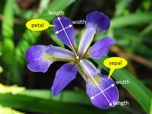
We’re trying to build an automatic flower classifier that, for measurements of a new flower returns the predicted species. To do this, we have a DataFrame with columns for species, petal width, petal length, sepal length, and sepal width. The species is what type of flower it is the petal and sepal are parts of the flower.

Note

This cell is hidden because it it not necessary for the narrative strucutre of our analysis, but it was useful for creating the next cell

Show code cell content Hide code cell content

iris_df.columns

Index(['sepal_length', 'sepal_width', 'petal_length', 'petal_width',
       'species'],
      dtype='object')

The species will be the target and the measurements will be the features. We want to predict the target from the features, the species from the measurements.

feature_vars = ['sepal_length', 'sepal_width', 'petal_length', 'petal_width']
target_var = 'species'

11.6. What does Naive Bayes do?

docs

Naive = indepdent features Bayes = most probable

Bayes Estimator

We can look at this data using a pair plot. It plots each pair of numerical variables in a grid of scatterplots and on the diagonal (where it would be a variable with itself) shows the distribution of that variable.

sns.pairplot(data=iris_df, hue=target_var)

<seaborn.axisgrid.PairGrid at 0x7fa60846aeb0>

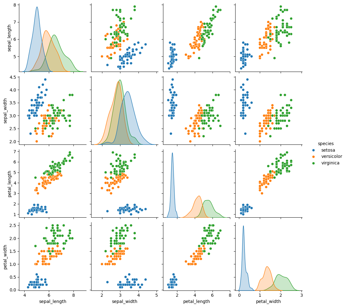
This data is reasonably separable beacuse the different species (indicated with colors in the plot) do not overlap much. We see that the features are distributed sort of like a normal, or Gaussian, distribution. In 2D a Gaussian distribution is like a hill, so we expect to see more points near the center and fewer on the edge of circle-ish blobs. These blobs are slightly live ovals, but not too skew.

This means that the assumptions of the Gaussian Naive Bayes model are met well enough we can expect the classifier to do well.

11.7. Separating Training and Test Data

To do machine learning, we split the data both sample wise (rows if tidy) and variable-wise (columns if tidy). First, we’ll designate the columns to use as features and as the target.

The features are the input that we wish to use to predict the target.

Next, we’ll use a sklearn function to split the data randomly into test and train portions.

Note

Here i set the random state. This means that the site will always have the same result even when this notebook is run over and over again.

Try downloading it (or adding random_state to your own code) and running it on your own computer.

X_train, X_test, y_train, y_test = train_test_split(iris_df[feature_vars],iris_df[target_var], random_state=0)

This function returns multiple values, the docs say that it returns twice as many as it is passed. We passed two separate things, the features and the labels separated, so we get train and test each for both.

Note

If you get different numbers fort the index than I do here or run the train test split multipe times and see things change, you have a different ranomd seed above.

X_train.head()

	sepal_length	sepal_width	petal_length	petal_width
61	5.9	3.0	4.2	1.5
92	5.8	2.6	4.0	1.2
112	6.8	3.0	5.5	2.1
2	4.7	3.2	1.3	0.2
141	6.9	3.1	5.1	2.3

We can see by default how many samples it puts the training set:

len(X_train)/len(iris_df)

0.7466666666666667

So by default we get a 75-25 split. But we can cahnget it.

11.8. Instantiating our Model Object

Next we will instantiate the object for our model. In sklearn they call these objects estimator. All estimators have a similar usage. First we instantiate the object and set any hyperparameters.

Instantiating the object says we are assuming a particular type of model. In this case Gaussian Naive Bayes. This sets several assumptions in one form:

• we assume data are Gaussian (normally) distributed

• the features are uncorrelated/independent (Naive)

• the best way to predict is to find the highest probability (Bayes)

this is one example of a Bayes Estimator

Further Reading

All of this is beyond the scope of this course, but may be of interest The Scikit Learn User Guide is a really good place to learn the details of machine learning. It is high quality documentation from both a statistical and computer science perspective of every element of the library.

The sklearn API describes how the library is structured and organized. Because the library is so popular (and it’s pretty well architected from a software perspective as well) if you are developing new machine learning techniques it’s good to make them sklearn compatible.

For example, IBM’s AIF360 is a package for doing fair machine learning which has a sklearn compatible interface. Scikit Learn documentation also includes a related projects page.

gnb = GaussianNB()

At this point the object is not very interesting

gnb.__dict__

{'priors': None, 'var_smoothing': 1e-09}

The fit method uses the data to learn the model’s parameters. In this case, a Gaussian distribution is characterized by a mean and variance; so the GNB classifier is characterized by one mean and one variance for each class (in 4d, like our data)

gnb.fit(X_train,y_train)

GaussianNB()

In a Jupyter environment, please rerun this cell to show the HTML representation or trust the notebook.
On GitHub, the HTML representation is unable to render, please try loading this page with nbviewer.org.

The attributes of the estimator object (gbn) describe the data (eg the class list) and the model’s parameters. The theta_ (\(\theta\)) represents the mean and the sigma_ (\(\sigma\)) represents the variance of the distributions.

gnb.__dict__

{'priors': None,
 'var_smoothing': 1e-09,
 'classes_': array(['setosa', 'versicolor', 'virginica'], dtype='<U10'),
 'feature_names_in_': array(['sepal_length', 'sepal_width', 'petal_length', 'petal_width'],
       dtype=object),
 'n_features_in_': 4,
 'epsilon_': 3.2135586734693885e-09,
 'theta_': array([[4.9972973 , 3.38918919, 1.45405405, 0.24054054],
        [5.91764706, 2.75882353, 4.19117647, 1.30882353],
        [6.66341463, 2.9902439 , 5.58292683, 2.03902439]]),
 'var_': array([[0.12242513, 0.14474799, 0.01978087, 0.01159971],
        [0.2649827 , 0.11124568, 0.22139274, 0.0408045 ],
        [0.4071981 , 0.11453897, 0.30483046, 0.06579417]]),
 'class_count_': array([37., 34., 41.]),
 'class_prior_': array([0.33035714, 0.30357143, 0.36607143])}

Once we fit, we can predict

y_pred = gnb.predict(X_test)

we get one prediciton for each sample.

len(y_pred), len(X_test)

(38, 38)

We can evaluate this using the score we learned last week

accuracy_score(y_test,y_pred)

1.0

or by checking it manually:

sum(y_pred ==y_test)/len(y_test)

1.0

Estimator objects also have a score method. If the estimator is a classifier, that score is accuracy. We will see that for other types of estimators it is different types.

gnb.score(X_test,y_test)

1.0

11.9. Questions After Class

Note

I used questions from previous semesters because few questions were asked.

11.9.1. Can you use machine learning for any type of data?

Yes the features for example could be an image instead of four numbers. It could also be text. The basic ideas are the same for more complex data, so we are going to spend a lot of time building your understanding of what ML is on simple data. Past students have successfully applied ML in more complex data after this course because once you have a good understanding of the core ideas, applying it to other forms of data is easier to learn on your own.

11.9.2. Can we check how well the model did using the y_test df?

we could compare them directly or using score that does.

y_pred == y_test

114    True
62     True
33     True
107    True
7      True
100    True
40     True
86     True
76     True
71     True
134    True
51     True
73     True
54     True
63     True
37     True
78     True
90     True
45     True
16     True
121    True
66     True
24     True
8      True
126    True
22     True
44     True
97     True
93     True
26     True
137    True
84     True
27     True
127    True
132    True
59     True
18     True
83     True
Name: species, dtype: bool

sum(y_pred == y_test)/len(y_test)

1.0

gnb.score(X_test,y_test)

1.0

We can also use any of the other metrics we saw, we’ll practice more on Wednesday

11.9.3. I want to know more about the the test_train_split() function

the docs are a good place to start.

11.9.4. Could we use the comparison stuff we’ve been learning to test the ML algorithm?

Yes!!

11.9.5. How should we set the random set we had for x_test to a specific group?

the random_state parameter will fix it.

11.9.6. Are there any good introductions to ScikitLearn that you are aware of?

Scikit Learn User Guide is the best one and they have a large example gallery.