
5. Visualization#
Warning
If your plots do not show, include this in any cell. The % signals that this is an
ipython magic. This one controls matplotlib. Jupyter uses the IPython python kernel.
import pandas as pd
import seaborn as sns
5.1. Summarizing Review#
We will start with the same dataset we hvae been working with
robusta_data_url = 'https://raw.githubusercontent.com/jldbc/coffee-quality-database/master/data/robusta_data_cleaned.csv'
robusta_df = pd.read_csv(robusta_data_url,index_col=0)
robusta_df.head(1)
| Species | Owner | Country.of.Origin | Farm.Name | Lot.Number | Mill | ICO.Number | Company | Altitude | Region | ... | Color | Category.Two.Defects | Expiration | Certification.Body | Certification.Address | Certification.Contact | unit_of_measurement | altitude_low_meters | altitude_high_meters | altitude_mean_meters | |
|---|---|---|---|---|---|---|---|---|---|---|---|---|---|---|---|---|---|---|---|---|---|
| 1 | Robusta | ankole coffee producers coop | Uganda | kyangundu cooperative society | NaN | ankole coffee producers | 0 | ankole coffee producers coop | 1488 | sheema south western | ... | Green | 2 | June 26th, 2015 | Uganda Coffee Development Authority | e36d0270932c3b657e96b7b0278dfd85dc0fe743 | 03077a1c6bac60e6f514691634a7f6eb5c85aae8 | m | 1488.0 | 1488.0 | 1488.0 |
1 rows × 43 columns
Is the robust coffee’s Mouthfeel or the Aftertaste more consistently scored in this dataset?
Why?
cols_to_compare = ['Mouthfeel', 'Aftertaste']
robusta_df[cols_to_compare].std()
Mouthfeel     0.725152
Aftertaste    0.342469
dtype: float64
from the lower std we can see that Aftertaste is more consistently rated.
We will use a larger dataset for more interesting plots.
arabica_data_url = 'https://raw.githubusercontent.com/jldbc/coffee-quality-database/master/data/arabica_data_cleaned.csv'
coffee_df = pd.read_csv(arabica_data_url,index_col=0)
coffee_df.head(1)
| Species | Owner | Country.of.Origin | Farm.Name | Lot.Number | Mill | ICO.Number | Company | Altitude | Region | ... | Color | Category.Two.Defects | Expiration | Certification.Body | Certification.Address | Certification.Contact | unit_of_measurement | altitude_low_meters | altitude_high_meters | altitude_mean_meters | |
|---|---|---|---|---|---|---|---|---|---|---|---|---|---|---|---|---|---|---|---|---|---|
| 1 | Arabica | metad plc | Ethiopia | metad plc | NaN | metad plc | 2014/2015 | metad agricultural developmet plc | 1950-2200 | guji-hambela | ... | Green | 0 | April 3rd, 2016 | METAD Agricultural Development plc | 309fcf77415a3661ae83e027f7e5f05dad786e44 | 19fef5a731de2db57d16da10287413f5f99bc2dd | m | 1950.0 | 2200.0 | 2075.0 |
1 rows × 43 columns
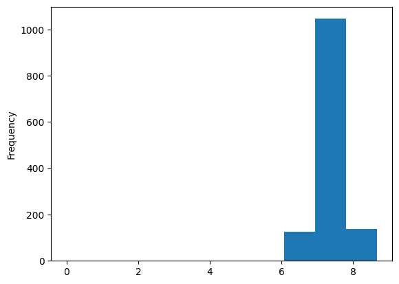
Recall, we can us built in plots in pandas.
coffee_df['Aftertaste'].plot(kind='hist')
<Axes: ylabel='Frequency'>
5.2. Plotting in Python#
matplotlib: low level plotting tools
seaborn: high level plotting with opinionated defaults
ggplot: plotting based on the ggplot library in R.
Pandas and seaborn use matplotlib under the hood.
Seaborn and ggplot both assume the data is set up as a DataFrame. Getting started with seaborn is the simplest, so we’ll use that.
There are lots of type of plots, we saw the basic patterns of how to use them and we’ve used a few types, but we cannot (and do not need to) go through every single type. There are general patterns that you can use that will help you think about what type of plot you might want and help you understand them to be able to customize plots.
[Seaborn’s main goal is opinionated defaults and flexible customization](https://seaborn.pydata.org/tutorial/introduction.html#opinionated-defaults-and-flexible-customization
5.2.1. Anatomy of a figure#
First is the matplotlib structure of a figure. BOth pandas and seaborn and other plotting libraries use matplotlib. Matplotlib was used in visualizing the first Black hole.
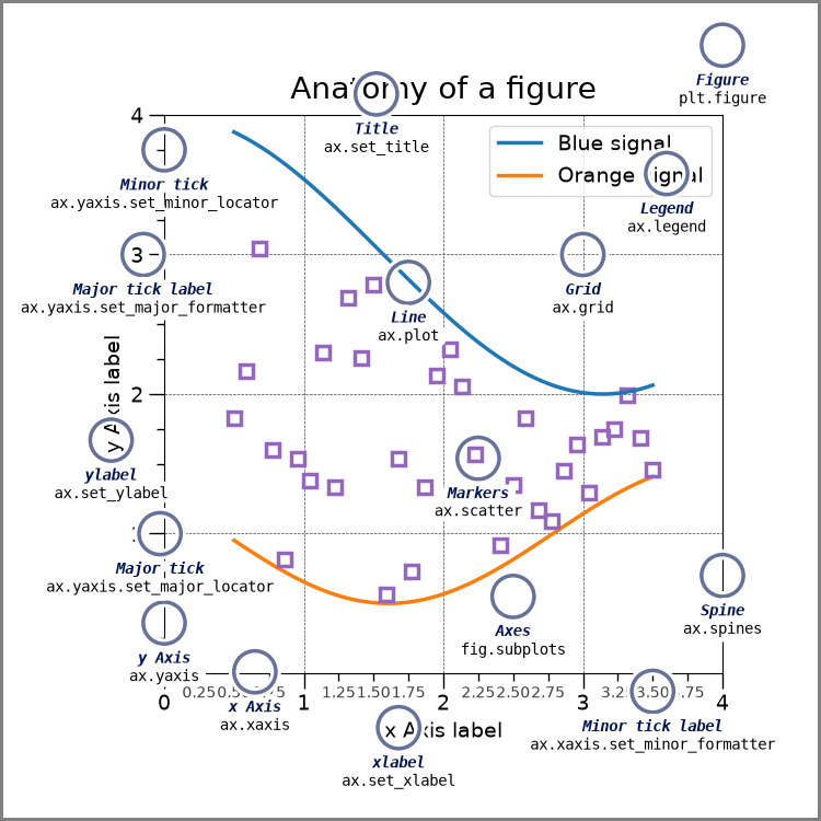
This is a lot of information, but these are good to know things. THe most important is the figure and the axes.
Try it Yourself
Make sure you can explain what is a figure and what are axes in your own words and why that distinction matters. Discuss in office hours if you are unsure.
that image was drawn with code and that page explains more.
5.2.2. Plotting Function types in Seaborn#
Seaborn has two levels or groups of plotting functions. Figure and axes. Figure level fucntions can plot with subplots.
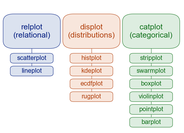
This is from thie overivew section of the official seaborn tutorial. It also includes a comparison of figure vs axes plotting.
The official introduction is also a good read.
5.2.3. More#
The seaborn gallery and matplotlib gallery are nice to look at too.
5.2.4. Styling in Seaborn#
Important
This was not covered in class, but can be helpful
Seaborn also lets us set a theme for visual styling This by default styles the plots to be more visually appealing
sns.set_theme(palette='colorblind')
the colorblind palette is more distinguishable under a variety fo colorblindness types. for more. Colorblind is a good default, but you can choose others that you like more too.
robusta_df.columns
Index(['Species', 'Owner', 'Country.of.Origin', 'Farm.Name', 'Lot.Number',
       'Mill', 'ICO.Number', 'Company', 'Altitude', 'Region', 'Producer',
       'Number.of.Bags', 'Bag.Weight', 'In.Country.Partner', 'Harvest.Year',
       'Grading.Date', 'Owner.1', 'Variety', 'Processing.Method',
       'Fragrance...Aroma', 'Flavor', 'Aftertaste', 'Salt...Acid',
       'Bitter...Sweet', 'Mouthfeel', 'Uniform.Cup', 'Clean.Cup', 'Balance',
       'Cupper.Points', 'Total.Cup.Points', 'Moisture', 'Category.One.Defects',
       'Quakers', 'Color', 'Category.Two.Defects', 'Expiration',
       'Certification.Body', 'Certification.Address', 'Certification.Contact',
       'unit_of_measurement', 'altitude_low_meters', 'altitude_high_meters',
       'altitude_mean_meters'],
      dtype='object')
coffee_df.columns
Index(['Species', 'Owner', 'Country.of.Origin', 'Farm.Name', 'Lot.Number',
       'Mill', 'ICO.Number', 'Company', 'Altitude', 'Region', 'Producer',
       'Number.of.Bags', 'Bag.Weight', 'In.Country.Partner', 'Harvest.Year',
       'Grading.Date', 'Owner.1', 'Variety', 'Processing.Method', 'Aroma',
       'Flavor', 'Aftertaste', 'Acidity', 'Body', 'Balance', 'Uniformity',
       'Clean.Cup', 'Sweetness', 'Cupper.Points', 'Total.Cup.Points',
       'Moisture', 'Category.One.Defects', 'Quakers', 'Color',
       'Category.Two.Defects', 'Expiration', 'Certification.Body',
       'Certification.Address', 'Certification.Contact', 'unit_of_measurement',
       'altitude_low_meters', 'altitude_high_meters', 'altitude_mean_meters'],
      dtype='object')
Important
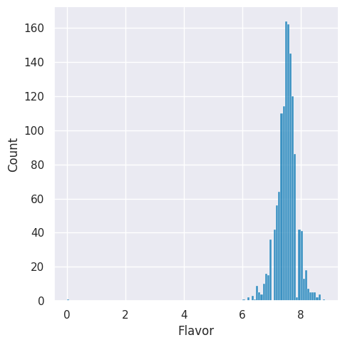
For seaborn the online documentation is immensely valuable. Every function’s page has basic documentation and lots of examples, so you can see how they use different paramters to modify plots visually. I strongly recommend reading it often. I recommend reading their tutorial too
sns.displot(data = coffee_df, x='Flavor')
<seaborn.axisgrid.FacetGrid at 0x7f3cd2879160>
Note explain the layout warning
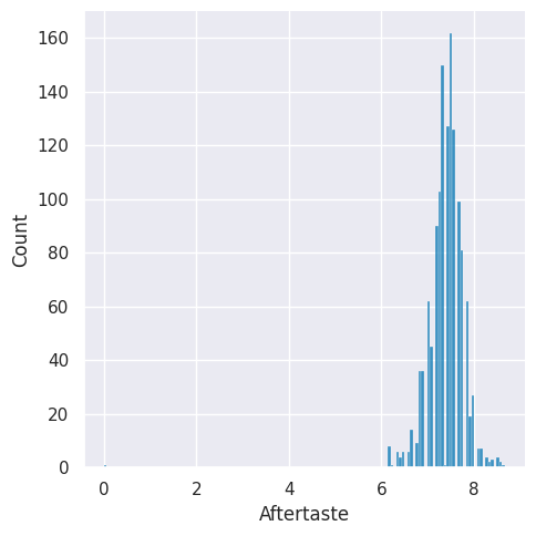
sns.displot(data = coffee_df, x='Aftertaste',)
<seaborn.axisgrid.FacetGrid at 0x7f3c87f8c160>
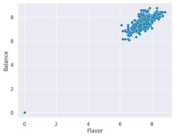
sns.scatterplot(data=coffee_df, x='Flavor', y='Balance')
<Axes: xlabel='Flavor', ylabel='Balance'>
sns.relplot(data=coffee_df, x='Flavor', y='Balance',)
<seaborn.axisgrid.FacetGrid at 0x7f3c87f902e0>
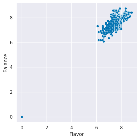
Plotting functions return an object that you can use to customize the plots further.
g = sns.relplot(data=coffee_df, x='Flavor', y='Balance',
           hue='Country.of.Origin',)
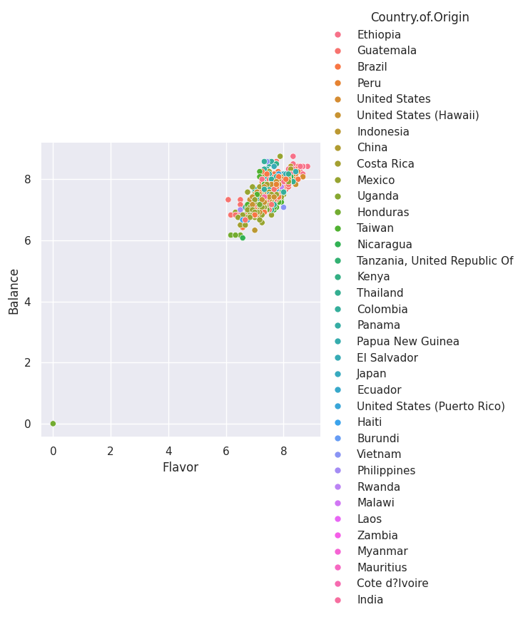
type(g)
seaborn.axisgrid.FacetGrid
g. # tab can show the options for attributes andmethods on this object
  Cell In[16], line 1
    g. # tab can show the options for attributes andmethods on this object
       ^
SyntaxError: invalid syntax
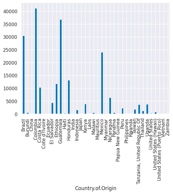
5.3. Bags per country#
How many bags of coffee are produced per country?
sns.catplot(data=coffee_df, x='Country.of.Origin',y='Number.of.Bags',
           kind='count');
---------------------------------------------------------------------------
ValueError                                Traceback (most recent call last)
Cell In[17], line 1
----> 1 sns.catplot(data=coffee_df, x='Country.of.Origin',y='Number.of.Bags',
      2            kind='count');

File /opt/hostedtoolcache/Python/3.8.18/x64/lib/python3.8/site-packages/seaborn/categorical.py:2764, in catplot(data, x, y, hue, row, col, kind, estimator, errorbar, n_boot, units, seed, order, hue_order, row_order, col_order, col_wrap, height, aspect, log_scale, native_scale, formatter, orient, color, palette, hue_norm, legend, legend_out, sharex, sharey, margin_titles, facet_kws, ci, **kwargs)
   2762         y = 1
   2763     elif x is not None and y is not None:
-> 2764         raise ValueError("Cannot pass values for both `x` and `y`.")
   2766 p = Plotter(
   2767     data=data,
   2768     variables=dict(x=x, y=y, hue=hue, row=row, col=col, units=units),
   (...)
   2774     legend=legend,
   2775 )
   2777 for var in ["row", "col"]:
   2778     # Handle faceting variables that lack name information

ValueError: Cannot pass values for both `x` and `y`.
coffee_df.shape
(1311, 43)
coffee_df.groupby('Country.of.Origin')['Number.of.Bags'].sum()
Country.of.Origin
Brazil                          30534
Burundi                           520
China                              55
Colombia                        41204
Costa Rica                      10354
Cote d?Ivoire                       2
Ecuador                             1
El Salvador                      4449
Ethiopia                        11761
Guatemala                       36868
Haiti                             390
Honduras                        13167
India                              20
Indonesia                        1658
Japan                              20
Kenya                            3971
Laos                               81
Malawi                            557
Mauritius                           1
Mexico                          24140
Myanmar                            10
Nicaragua                        6406
Panama                            537
Papua New Guinea                    7
Peru                             2336
Philippines                       259
Rwanda                            150
Taiwan                           1914
Tanzania, United Republic Of     3760
Thailand                         1310
Uganda                           3868
United States                     361
United States (Hawaii)            833
United States (Puerto Rico)        71
Vietnam                            10
Zambia                             13
Name: Number.of.Bags, dtype: int64
country_grouped = coffee_df.groupby('Country.of.Origin')
country_grouped
<pandas.core.groupby.generic.DataFrameGroupBy object at 0x7f3c879e2d30>
bag_total_dict = {}

for country,df in country_grouped:
    tot_bags =  df['Number.of.Bags'].sum()
    bag_total_dict[country] = tot_bags

pd.DataFrame.from_dict(bag_total_dict, orient='index',
                           columns = ['Number.of.Bags.Sum'])
| Number.of.Bags.Sum | |
|---|---|
| Brazil | 30534 |
| Burundi | 520 |
| China | 55 |
| Colombia | 41204 |
| Costa Rica | 10354 |
| Cote d?Ivoire | 2 |
| Ecuador | 1 |
| El Salvador | 4449 |
| Ethiopia | 11761 |
| Guatemala | 36868 |
| Haiti | 390 |
| Honduras | 13167 |
| India | 20 |
| Indonesia | 1658 |
| Japan | 20 |
| Kenya | 3971 |
| Laos | 81 |
| Malawi | 557 |
| Mauritius | 1 |
| Mexico | 24140 |
| Myanmar | 10 |
| Nicaragua | 6406 |
| Panama | 537 |
| Papua New Guinea | 7 |
| Peru | 2336 |
| Philippines | 259 |
| Rwanda | 150 |
| Taiwan | 1914 |
| Tanzania, United Republic Of | 3760 |
| Thailand | 1310 |
| Uganda | 3868 |
| United States | 361 |
| United States (Hawaii) | 833 |
| United States (Puerto Rico) | 71 |
| Vietnam | 10 |
| Zambia | 13 |
'a b'.split(' ')
['a', 'b']
a,b = 'a b'.split(' ')
a
'a'
b
'b'
bags_per_country_df = coffee_df.groupby('Country.of.Origin')['Number.of.Bags'].sum()
bags_per_country_df.plot(kind='bar')
<Axes: xlabel='Country.of.Origin'>
coffee_df.columns
Index(['Species', 'Owner', 'Country.of.Origin', 'Farm.Name', 'Lot.Number',
       'Mill', 'ICO.Number', 'Company', 'Altitude', 'Region', 'Producer',
       'Number.of.Bags', 'Bag.Weight', 'In.Country.Partner', 'Harvest.Year',
       'Grading.Date', 'Owner.1', 'Variety', 'Processing.Method', 'Aroma',
       'Flavor', 'Aftertaste', 'Acidity', 'Body', 'Balance', 'Uniformity',
       'Clean.Cup', 'Sweetness', 'Cupper.Points', 'Total.Cup.Points',
       'Moisture', 'Category.One.Defects', 'Quakers', 'Color',
       'Category.Two.Defects', 'Expiration', 'Certification.Body',
       'Certification.Address', 'Certification.Contact', 'unit_of_measurement',
       'altitude_low_meters', 'altitude_high_meters', 'altitude_mean_meters'],
      dtype='object')
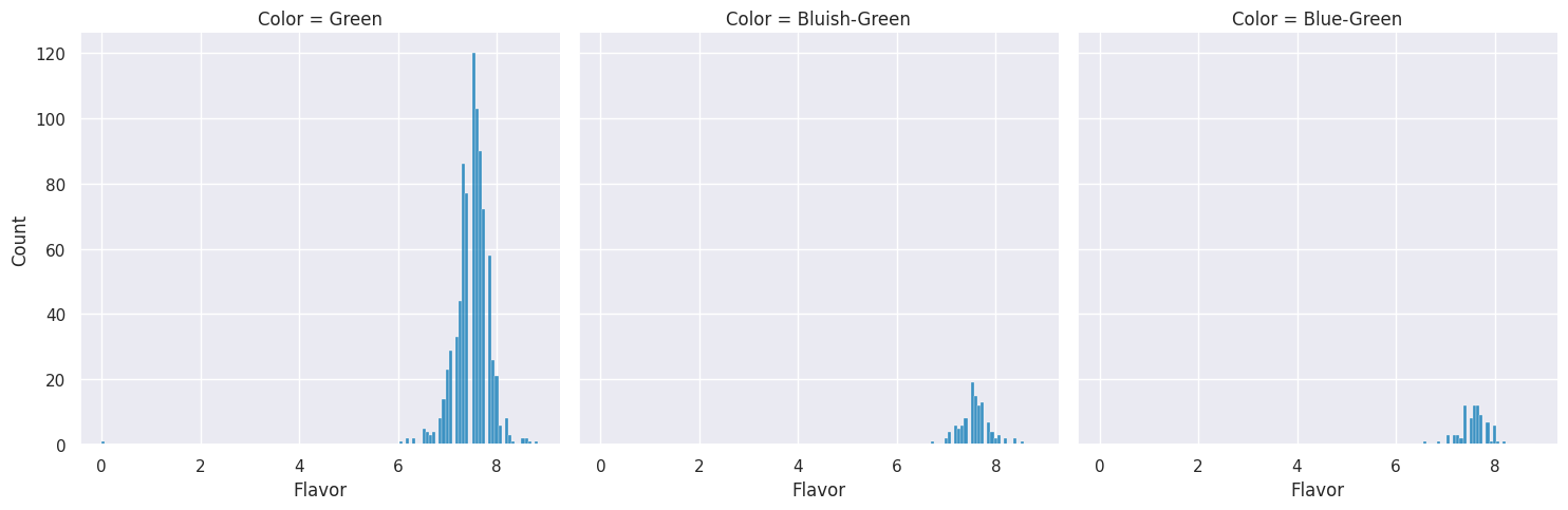
flavor_by_color = coffee_df.groupby('Color')['Flavor']
flavor_by_color.mean()
Color
Blue-Green      7.577317
Bluish-Green    7.581518
Green           7.491482
Name: Flavor, dtype: float64
flavor_by_color.std()
Color
Blue-Green      0.276513
Bluish-Green    0.301241
Green           0.413324
Name: Flavor, dtype: float64
sns.displot(data=coffee_df, x='Flavor',col='Color' )
<seaborn.axisgrid.FacetGrid at 0x7f3c7fec7f10>
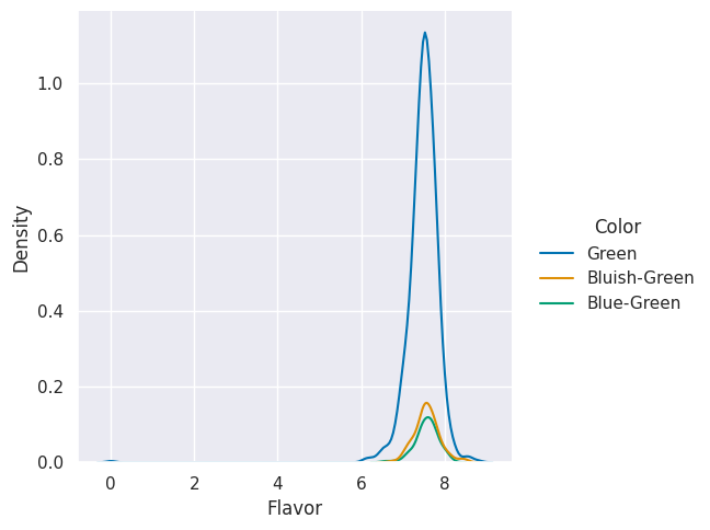
sns.displot(data=coffee_df, x='Flavor',hue='Color' ,kind='kde')
<seaborn.axisgrid.FacetGrid at 0x7f3c7ff34370>
5.4. Filtering a DataFrame#
Now, we’ll take just the country names out
How does color vary by country of origin for the top 10 countries with the most ratings?
df_country = coffee_df['Country.of.Origin'].value_counts()
top_countries = df_country[:10].index
top_countries
Index(['Mexico', 'Colombia', 'Guatemala', 'Brazil', 'Taiwan',
       'United States (Hawaii)', 'Honduras', 'Costa Rica', 'Ethiopia',
       'Tanzania, United Republic Of'],
      dtype='object', name='Country.of.Origin')
5.4.1. Filtering with a lambda and the apply method?#
check_top_country = lambda r: r['Country.of.Origin'] in top_countries
'Mexico' in top_countries
True
'USA' in top_countries
False
top_country_df = coffee_df[coffee_df.apply(check_top_country,axis=1)]
5.4.2. Filtering with isin#
and we can use that to filter the original DataFrame. To do this, we use isin to check each element in the 'Country.of.Origin' column is in that list.
coffee_df['Country.of.Origin'].isin(top_countries)
1        True
2        True
3        True
4        True
5        True
        ...
1307     True
1308    False
1309    False
1310     True
1312     True
Name: Country.of.Origin, Length: 1311, dtype: bool
This is roughly equivalent to:
[country in top_countries for country in coffee_df['Country.of.Origin'] ]
[True,
 True,
 True,
 True,
 True,
 True,
 False,
 True,
 True,
 True,
 True,
 False,
 False,
 True,
 True,
 False,
 False,
 True,
 False,
 True,
 False,
 True,
 True,
 False,
 True,
 True,
 True,
 False,
 True,
 True,
 False,
 True,
 True,
 True,
 True,
 False,
 True,
 True,
 True,
 False,
 False,
 True,
 True,
 True,
 False,
 True,
 False,
 True,
 False,
 False,
 True,
 True,
 True,
 False,
 True,
 False,
 True,
 True,
 True,
 True,
 False,
 False,
 False,
 False,
 True,
 False,
 False,
 True,
 False,
 True,
 True,
 False,
 True,
 True,
 False,
 False,
 True,
 True,
 True,
 False,
 False,
 True,
 True,
 True,
 True,
 True,
 False,
 True,
 True,
 True,
 True,
 True,
 True,
 True,
 True,
 True,
 False,
 True,
 True,
 True,
 False,
 False,
 True,
 True,
 True,
 True,
 True,
 True,
 True,
 True,
 True,
 True,
 True,
 True,
 False,
 True,
 False,
 True,
 True,
 True,
 False,
 False,
 True,
 False,
 False,
 False,
 False,
 False,
 True,
 True,
 True,
 True,
 True,
 True,
 True,
 True,
 True,
 False,
 True,
 True,
 True,
 False,
 False,
 True,
 False,
 True,
 True,
 False,
 True,
 True,
 True,
 True,
 False,
 True,
 True,
 True,
 True,
 True,
 True,
 False,
 False,
 True,
 True,
 False,
 True,
 False,
 True,
 True,
 True,
 True,
 True,
 True,
 False,
 True,
 True,
 True,
 True,
 True,
 True,
 False,
 True,
 True,
 True,
 True,
 True,
 True,
 True,
 True,
 True,
 True,
 True,
 True,
 False,
 True,
 True,
 True,
 False,
 True,
 True,
 True,
 True,
 True,
 True,
 True,
 True,
 True,
 True,
 True,
 True,
 False,
 True,
 True,
 True,
 True,
 True,
 True,
 True,
 False,
 True,
 True,
 True,
 True,
 True,
 True,
 False,
 True,
 True,
 False,
 True,
 True,
 False,
 False,
 True,
 True,
 True,
 True,
 True,
 True,
 True,
 True,
 True,
 True,
 True,
 True,
 True,
 True,
 True,
 True,
 True,
 True,
 True,
 True,
 True,
 False,
 False,
 False,
 False,
 False,
 True,
 True,
 False,
 True,
 True,
 True,
 True,
 True,
 True,
 True,
 True,
 True,
 True,
 True,
 True,
 True,
 True,
 True,
 True,
 True,
 True,
 True,
 True,
 True,
 True,
 True,
 True,
 True,
 False,
 True,
 True,
 True,
 True,
 True,
 False,
 False,
 True,
 False,
 True,
 True,
 True,
 True,
 False,
 True,
 False,
 False,
 True,
 True,
 True,
 True,
 True,
 True,
 True,
 True,
 True,
 True,
 True,
 False,
 True,
 False,
 True,
 True,
 True,
 False,
 True,
 True,
 True,
 True,
 True,
 True,
 True,
 True,
 True,
 True,
 False,
 True,
 True,
 True,
 True,
 True,
 False,
 True,
 True,
 True,
 False,
 True,
 True,
 True,
 True,
 True,
 True,
 True,
 True,
 True,
 True,
 True,
 True,
 True,
 True,
 True,
 False,
 True,
 True,
 True,
 True,
 True,
 True,
 True,
 True,
 True,
 True,
 True,
 True,
 True,
 True,
 True,
 False,
 True,
 True,
 True,
 True,
 True,
 False,
 False,
 False,
 True,
 True,
 True,
 True,
 True,
 True,
 True,
 True,
 True,
 True,
 True,
 False,
 True,
 True,
 True,
 True,
 True,
 True,
 True,
 True,
 True,
 True,
 True,
 True,
 False,
 False,
 True,
 True,
 True,
 False,
 True,
 True,
 True,
 True,
 True,
 True,
 True,
 False,
 True,
 True,
 True,
 True,
 True,
 True,
 True,
 True,
 True,
 True,
 True,
 True,
 True,
 True,
 True,
 True,
 True,
 True,
 True,
 True,
 True,
 True,
 False,
 False,
 True,
 True,
 False,
 False,
 False,
 True,
 True,
 False,
 False,
 True,
 True,
 False,
 True,
 True,
 True,
 True,
 True,
 True,
 True,
 True,
 True,
 True,
 True,
 True,
 True,
 True,
 True,
 True,
 True,
 True,
 True,
 False,
 True,
 True,
 True,
 True,
 True,
 True,
 True,
 True,
 True,
 True,
 True,
 True,
 True,
 True,
 True,
 True,
 True,
 False,
 True,
 True,
 True,
 True,
 False,
 False,
 True,
 False,
 True,
 True,
 True,
 True,
 True,
 False,
 False,
 True,
 True,
 True,
 True,
 True,
 True,
 True,
 True,
 True,
 True,
 True,
 True,
 True,
 True,
 True,
 True,
 False,
 True,
 True,
 True,
 True,
 False,
 False,
 True,
 False,
 True,
 True,
 True,
 True,
 False,
 False,
 True,
 True,
 True,
 False,
 False,
 True,
 True,
 True,
 True,
 True,
 True,
 True,
 True,
 False,
 True,
 True,
 True,
 False,
 False,
 True,
 True,
 False,
 False,
 False,
 True,
 True,
 True,
 False,
 True,
 True,
 True,
 True,
 True,
 True,
 True,
 True,
 False,
 True,
 True,
 True,
 True,
 True,
 False,
 True,
 True,
 False,
 True,
 True,
 True,
 False,
 False,
 True,
 False,
 True,
 True,
 True,
 True,
 True,
 True,
 True,
 True,
 True,
 True,
 True,
 False,
 True,
 True,
 True,
 False,
 False,
 True,
 True,
 True,
 True,
 True,
 True,
 True,
 True,
 False,
 True,
 False,
 True,
 False,
 True,
 False,
 True,
 True,
 True,
 True,
 True,
 True,
 True,
 True,
 True,
 True,
 True,
 True,
 False,
 False,
 False,
 True,
 False,
 True,
 True,
 True,
 True,
 True,
 True,
 True,
 True,
 True,
 True,
 True,
 False,
 True,
 True,
 False,
 False,
 True,
 True,
 True,
 True,
 True,
 True,
 True,
 True,
 True,
 True,
 True,
 True,
 True,
 True,
 True,
 True,
 True,
 True,
 True,
 True,
 True,
 False,
 True,
 True,
 True,
 True,
 True,
 True,
 False,
 True,
 True,
 True,
 True,
 True,
 True,
 True,
 True,
 True,
 True,
 True,
 True,
 True,
 True,
 True,
 True,
 True,
 True,
 True,
 True,
 True,
 True,
 True,
 False,
 True,
 True,
 True,
 False,
 True,
 True,
 True,
 True,
 True,
 True,
 True,
 True,
 True,
 True,
 True,
 True,
 True,
 True,
 True,
 True,
 True,
 True,
 True,
 True,
 True,
 True,
 False,
 True,
 False,
 True,
 True,
 True,
 True,
 True,
 True,
 True,
 True,
 False,
 True,
 True,
 True,
 True,
 True,
 True,
 True,
 True,
 False,
 True,
 True,
 True,
 False,
 True,
 True,
 True,
 True,
 True,
 True,
 True,
 True,
 True,
 True,
 True,
 True,
 True,
 True,
 False,
 True,
 True,
 True,
 True,
 True,
 True,
 True,
 True,
 True,
 True,
 True,
 True,
 False,
 True,
 True,
 True,
 True,
 True,
 True,
 True,
 False,
 True,
 False,
 True,
 False,
 True,
 True,
 True,
 True,
 True,
 True,
 True,
 True,
 True,
 True,
 True,
 True,
 True,
 True,
 True,
 True,
 False,
 True,
 True,
 False,
 False,
 True,
 True,
 True,
 True,
 True,
 True,
 True,
 True,
 True,
 True,
 True,
 True,
 False,
 True,
 True,
 True,
 False,
 True,
 True,
 True,
 True,
 False,
 False,
 True,
 True,
 True,
 True,
 True,
 True,
 True,
 True,
 True,
 True,
 True,
 True,
 True,
 False,
 True,
 True,
 True,
 True,
 True,
 True,
 True,
 True,
 True,
 True,
 True,
 True,
 True,
 True,
 False,
 True,
 True,
 True,
 True,
 True,
 False,
 True,
 True,
 True,
 True,
 True,
 True,
 True,
 True,
 True,
 True,
 True,
 True,
 True,
 True,
 True,
 True,
 True,
 True,
 False,
 True,
 True,
 True,
 True,
 True,
 True,
 False,
 False,
 True,
 True,
 False,
 True,
 True,
 True,
 False,
 True,
 False,
 True,
 True,
 True,
 False,
 True,
 True,
 True,
 True,
 True,
 True,
 True,
 False,
 True,
 True,
 True,
 True,
 True,
 True,
 True,
 True,
 True,
 False,
 True,
 True,
 True,
 False,
 True,
 True,
 True,
 True,
 True,
 True,
 True,
 True,
 True,
 True,
 True,
 True,
 False,
 False,
 True,
 True,
 True,
 True,
 True,
 True,
 False,
 True,
 True,
 True,
 True,
 True,
 True,
 False,
 True,
 True,
 True,
 True,
 False,
 False,
 True,
 False,
 True,
 True,
 True,
 True,
 True,
 True,
 True,
 True,
 False,
 False,
 True,
 True,
 False,
 True,
 True,
 True,
 True,
 True,
 True,
 False,
 ...]
except this builds a list and the pandas way makes a pd.Series object. The Python in operator is really helpful to know and pandas offers us an isin method to get that type of pattern.
In a more basic programming format this process would be two separate loops worth of work.
c_in = []
# iterate over the country of each rating
for country in coffee_df['Country.of.Origin']:
    # make a false temp value
    cur_search = False
    # iterate over top countries
    for tc in top_countries:
        # flip the value if the current top & rating cofee match
        if tc==country:
            cur_search = True
    # save the result of the search
    c_in.append(cur_search)
Try it yourself
Run these versions and confirm for yourself that they are the same.
With that list of booleans, we can then mask the original DataFrame. This keeps only the value where the inner quantity is True
top_coffee_df = coffee_df[coffee_df['Country.of.Origin'].isin(top_countries)]
top_coffee_df.head(1)
| Species | Owner | Country.of.Origin | Farm.Name | Lot.Number | Mill | ICO.Number | Company | Altitude | Region | ... | Color | Category.Two.Defects | Expiration | Certification.Body | Certification.Address | Certification.Contact | unit_of_measurement | altitude_low_meters | altitude_high_meters | altitude_mean_meters | |
|---|---|---|---|---|---|---|---|---|---|---|---|---|---|---|---|---|---|---|---|---|---|
| 1 | Arabica | metad plc | Ethiopia | metad plc | NaN | metad plc | 2014/2015 | metad agricultural developmet plc | 1950-2200 | guji-hambela | ... | Green | 0 | April 3rd, 2016 | METAD Agricultural Development plc | 309fcf77415a3661ae83e027f7e5f05dad786e44 | 19fef5a731de2db57d16da10287413f5f99bc2dd | m | 1950.0 | 2200.0 | 2075.0 |
1 rows × 43 columns
top_coffee_df.shape, coffee_df.shape
((1068, 43), (1311, 43))
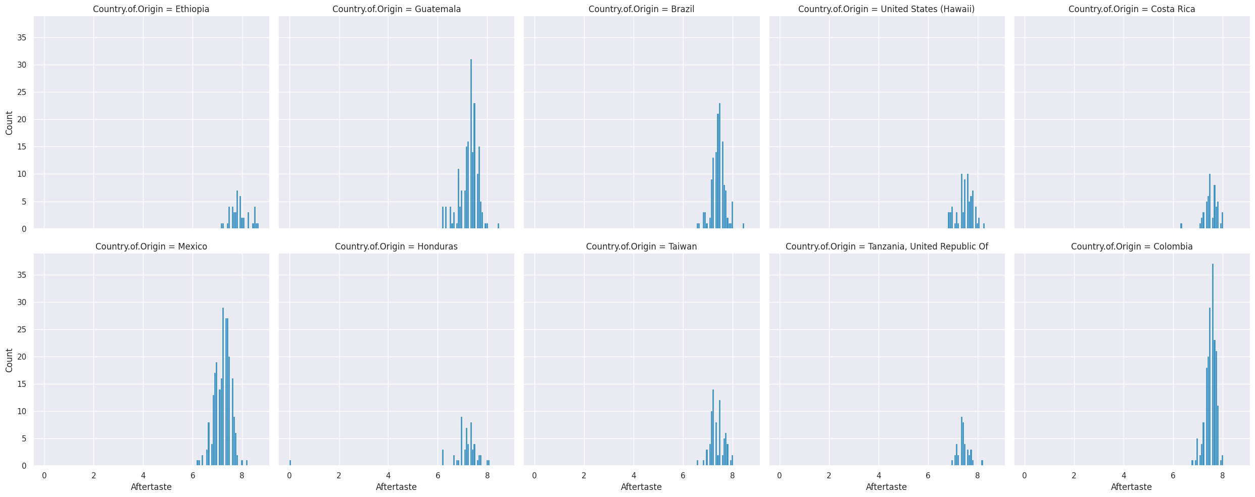
sns.displot(data=top_coffee_df,x='Aftertaste', col='Country.of.Origin',col_wrap=5)
<seaborn.axisgrid.FacetGrid at 0x7f3cd2474cd0>
5.5. Variable types and data types#
Related but not the same.
Data types are literal, related to the representation in the computer.
For exmaple, int16, int32, int64
We can also have mathematical types of numbers
Integers can be positive, 0, or negative.
Reals are continuous, infinite possibilities.
Variable types are about the meaning in a conceptual sense.
categorical (can take a discrete number of values, could be used to group data, could be a string or integer; unordered)
continuous (can take on any possible value, always a number)
binary (like data type boolean, but could be represented as yes/no, true/false, or 1/0, could be categorical also, but often makes sense to calculate rates)
ordinal (ordered, but appropriately categorical)
we’ll focus on the first two most of the time. Some values that are technically only integers range high enough that we treat them more like continuous most of the time.
5.6. Questions After Class#
5.6.1. how can I use data to make different graphs?#
You can use the help function on any of the plot functions we have seen. You can also use the documentation.
The seaborn gallery is a good place to get ideas
5.6.2. Will we learn about different types of graphs?#
We will use a few more types in class, but also you will probably use the documentation to learn more types. The seaborn gallery is a good place to start.
5.6.3. What are the advantages with work with the lambda function?#
The lambda function is convenient because it is defined on one line.
5.6.4. Is a lambda function similar to an arrow function in Javascript?#
It does look similar, but I am not an expert in javascipt.
5.6.5. How do you decide on the best graphs to use for each piece of data?#
Different types of plots make different conclusions easy to see.
5.6.6. why do you use axis = 1 for the check_top_countries#
5.6.7. could you do group by instead of value counts for the last question?#
yes