
12. Understanding Classification#
Today we are going to work on understandign what happens when a classifier makes
Important
You can provide feedback on the course so far
import pandas as pd
import seaborn as sns
from sklearn import tree
import matplotlib.pyplot as plt
from sklearn.model_selection import train_test_split
from sklearn.naive_bayes import GaussianNB
from sklearn import metrics
sns.set_theme(palette='colorblind') # this improves contrast

from sklearn.metrics import confusion_matrix, classification_report
Our goal is to predict the species from the measurements. Set up the problem by putting the variables in the correct roles (features and target) so that train test split will work.
iris_df = sns.load_dataset('iris')
Today we will use a different random state, recall that the random_state is like a name for the sequence of psuedo random numbers that it will use.
# dataset vars:
# 'petal_width',  'sepal_length','species', 'sepal_width','petal_length',
feature_vars = ['petal_width',  'sepal_length', 'sepal_width','petal_length']
target_var = 'species'
X_train, X_test, y_train, y_test = train_test_split(iris_df[feature_vars],
                                                    iris_df[target_var],random_state=3)
Again, we will plot the data with the target as the colors
sns.pairplot(data = iris_df, hue='species')
<seaborn.axisgrid.PairGrid at 0x7f7d5cb9b310>
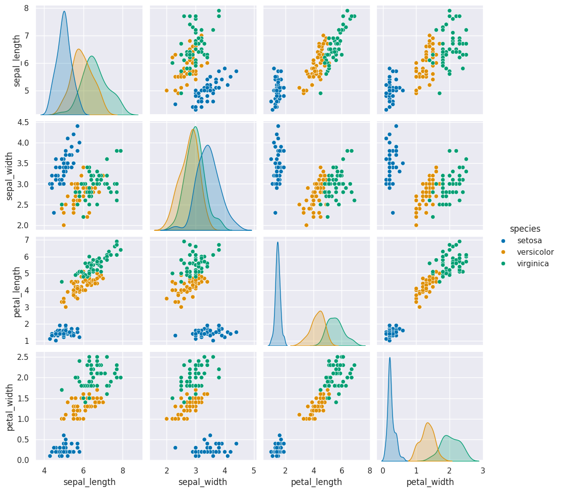
We notice that this data meets the assumptions of our model:
it is separable (for all classification)
the classes are each one blob that is roughly a circle or oval (gaussian)
the ovals are not too
gnb = GaussianNB()
gnb.fit(X_train,y_train)
GaussianNB()In a Jupyter environment, please rerun this cell to show the HTML representation or trust the notebook.
On GitHub, the HTML representation is unable to render, please try loading this page with nbviewer.org.
GaussianNB()
y_pred = gnb.predict(X_test)
gnb.score(X_test,y_test)
0.9736842105263158
We can also get a report with a few metrics.
Recall is the percent of each species that were predicted correctly.
Precision is the percent of the ones predicted to be in a species that are truly that species.
the F1 score is combination of the two
print(classification_report(y_test,y_pred))
              precision    recall  f1-score   support

      setosa       1.00      1.00      1.00        15
  versicolor       1.00      0.92      0.96        12
   virginica       0.92      1.00      0.96        11

    accuracy                           0.97        38
   macro avg       0.97      0.97      0.97        38
weighted avg       0.98      0.97      0.97        38
y_test.value_counts()
species
setosa        15
versicolor    12
virginica     11
Name: count, dtype: int64
confusion_matrix(y_test,y_pred)
array([[15,  0,  0],
       [ 0, 11,  1],
       [ 0,  0, 11]])
gnb.__dict__
{'priors': None,
 'var_smoothing': 1e-09,
 'classes_': array(['setosa', 'versicolor', 'virginica'], dtype='<U10'),
 'feature_names_in_': array(['petal_width', 'sepal_length', 'sepal_width', 'petal_length'],
       dtype=object),
 'n_features_in_': 4,
 'epsilon_': 2.9996867028061227e-09,
 'theta_': array([[0.24      , 5.04285714, 3.46285714, 1.46571429],
        [1.32631579, 5.89210526, 2.77894737, 4.23947368],
        [2.00769231, 6.54358974, 2.98461538, 5.53589744]]),
 'var_': array([[0.01268572, 0.0767347 , 0.09604898, 0.02911021],
        [0.03878117, 0.21862189, 0.10376732, 0.21186288],
        [0.06635109, 0.39425378, 0.10540434, 0.29204471]]),
 'class_count_': array([35., 38., 39.]),
 'class_prior_': array([0.3125    , 0.33928571, 0.34821429])}
import numpy as np
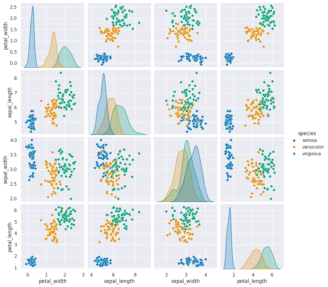
12.1. What does a generative model mean?#
To do this, we extract the mean and variance parameters from the model
(gnb.theta_,gnb.sigma_) and zip them together to create an iterable object
that in each iteration returns one value from each list (for th, sig in zip(gnb.theta_,gnb.sigma_)).
We do this inside of a list comprehension and for each th,sig where th is
from gnb.theta_ and sig is from gnb.sigma_ we use np.random.multivariate_normal
to get 20 samples. In a general multivariate normal distribution the second parameter is actually a covariance
matrix. This describes both the variance of each individual feature and the
correlation of the features. Since Naive Bayes is Naive it assumes the features
are independent or have 0 correlation. So, to create the matrix from the vector
of variances we multiply by np.eye(4) which is the identity matrix or a matrix
with 1 on the diagonal and 0 elsewhere. Finally we stack the groups for each
species together with np.concatenate (like pd.concat but works on numpy objects
and np.random.multivariate_normal returns numpy arrays not data frames) and put all of that in a
DataFrame using the feature names as the columns.
Then we add a species column, by repeating each species 20 times
[c]*N for c in gnb.classes_ and then unpack that into a single list instead of
as list of lists.
N = 50
gnb_df = pd.DataFrame(np.concatenate([np.random.multivariate_normal(th, sig*np.eye(4),N)
                 for th, sig in zip(gnb.theta_,gnb.var_)]),
                 columns = gnb.feature_names_in_)
gnb_df['species'] = [ci for cl in [[c]*N for c in gnb.classes_] for ci in cl]
sns.pairplot(data =gnb_df, hue='species')
<seaborn.axisgrid.PairGrid at 0x7f7d57d3aa60>
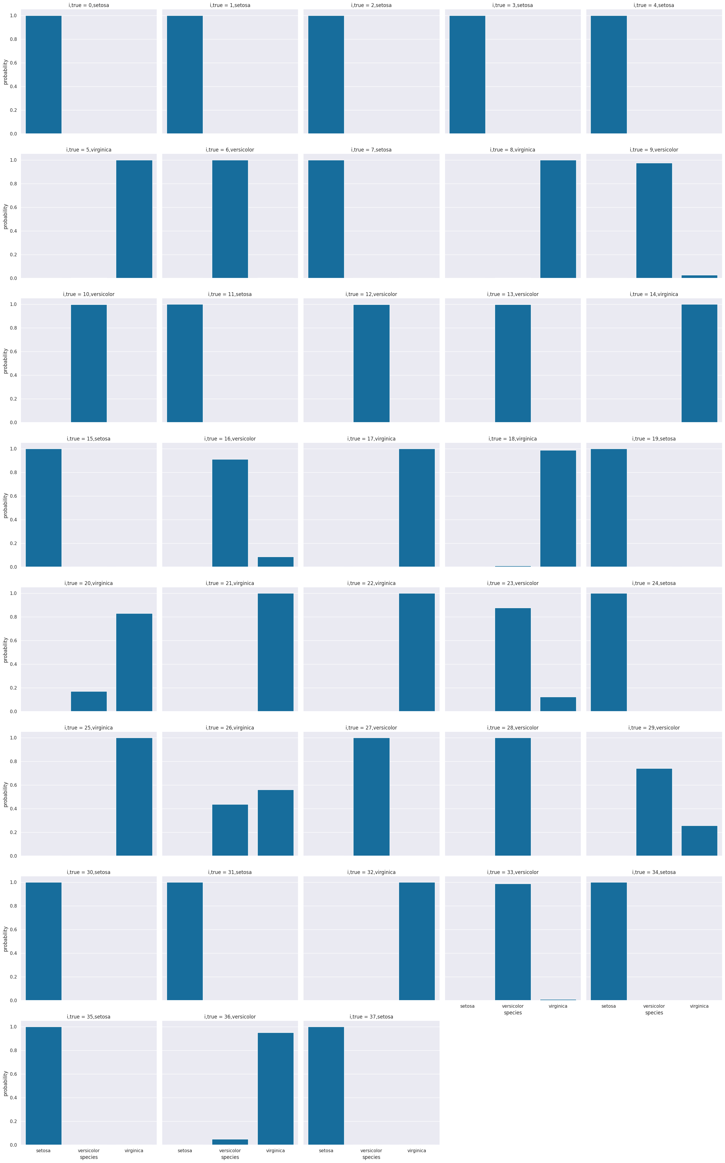
12.2. How does it make the predictions?#
gnb.predict_proba(X_test)
array([[1.00000000e+000, 3.10850430e-018, 9.83936388e-027],
       [1.00000000e+000, 2.17607686e-017, 6.11974996e-026],
       [1.00000000e+000, 2.45846863e-014, 9.60562575e-023],
       [1.00000000e+000, 4.29382017e-016, 8.65569962e-025],
       [1.00000000e+000, 5.49915897e-016, 2.38180484e-023],
       [1.99870101e-311, 1.36174299e-013, 1.00000000e+000],
       [2.69395984e-069, 9.99960647e-001, 3.93530354e-005],
       [1.00000000e+000, 1.40826499e-017, 5.89539964e-026],
       [1.08156958e-173, 1.40618746e-003, 9.98593813e-001],
       [2.90745994e-094, 9.75192625e-001, 2.48073750e-002],
       [5.39591648e-072, 9.99825700e-001, 1.74300433e-004],
       [1.00000000e+000, 5.38453222e-018, 1.35082184e-026],
       [1.30426983e-066, 9.99973771e-001, 2.62288452e-005],
       [6.11553492e-070, 9.99973058e-001, 2.69419127e-005],
       [2.01494877e-214, 4.34577051e-009, 9.99999996e-001],
       [1.00000000e+000, 5.75883870e-018, 2.19570953e-026],
       [1.15708888e-120, 9.13375722e-001, 8.66242784e-002],
       [1.35987974e-251, 2.26297317e-011, 1.00000000e+000],
       [5.67885061e-148, 1.14141144e-002, 9.88585886e-001],
       [1.00000000e+000, 1.36229423e-018, 5.09772462e-027],
       [2.60919798e-128, 1.70228595e-001, 8.29771405e-001],
       [2.54851174e-189, 2.95677415e-006, 9.99997043e-001],
       [3.04997634e-180, 3.40898084e-007, 9.99999659e-001],
       [2.00705701e-114, 8.76744267e-001, 1.23255733e-001],
       [1.00000000e+000, 2.97690385e-014, 4.03753917e-022],
       [2.46428706e-258, 9.61343301e-013, 1.00000000e+000],
       [1.52504682e-153, 4.39107652e-001, 5.60892348e-001],
       [8.50956394e-064, 9.99989920e-001, 1.00798872e-005],
       [1.15904764e-034, 9.99999826e-001, 1.73844955e-007],
       [5.34461569e-112, 7.42611536e-001, 2.57388464e-001],
       [1.00000000e+000, 1.76204469e-018, 3.45582363e-026],
       [1.00000000e+000, 1.05535449e-014, 7.37686742e-023],
       [3.87070789e-184, 3.08105361e-006, 9.99996919e-001],
       [2.82918552e-099, 9.88848742e-001, 1.11512583e-002],
       [1.00000000e+000, 2.84646765e-017, 6.28162840e-026],
       [1.00000000e+000, 7.38253736e-018, 3.74617670e-026],
       [6.06665872e-137, 4.97058492e-002, 9.50294151e-001],
       [1.00000000e+000, 1.30813624e-014, 6.57792025e-024]])
# make the probabilities into a dataframe labeled with classes & make the index a separate column
prob_df = pd.DataFrame(data = gnb.predict_proba(X_test), columns = gnb.classes_ ).reset_index()
# add the predictions
prob_df['predicted_species'] = y_pred
prob_df['true_species'] = y_test.values
# for plotting, make a column that combines the index & prediction
pred_text = lambda r: str( r['index']) + ',' + r['predicted_species']
prob_df['i,pred'] = prob_df.apply(pred_text,axis=1)
# same for ground truth
true_text = lambda r: str( r['index']) + ',' + r['true_species']
prob_df['correct'] = prob_df['predicted_species'] == prob_df['true_species']
# a dd a column for which are correct
prob_df['i,true'] = prob_df.apply(true_text,axis=1)
prob_df_melted = prob_df.melt(id_vars =[ 'index', 'predicted_species','true_species','i,pred','i,true','correct'],value_vars = gnb.classes_,
                             var_name = target_var, value_name = 'probability')
prob_df_melted.head()
| index | predicted_species | true_species | i,pred | i,true | correct | species | probability | |
|---|---|---|---|---|---|---|---|---|
| 0 | 0 | setosa | setosa | 0,setosa | 0,setosa | True | setosa | 1.0 |
| 1 | 1 | setosa | setosa | 1,setosa | 1,setosa | True | setosa | 1.0 |
| 2 | 2 | setosa | setosa | 2,setosa | 2,setosa | True | setosa | 1.0 |
| 3 | 3 | setosa | setosa | 3,setosa | 3,setosa | True | setosa | 1.0 |
| 4 | 4 | setosa | setosa | 4,setosa | 4,setosa | True | setosa | 1.0 |
# plot a bar graph for each point labeled with the prediction
sns.catplot(data =prob_df_melted, x = 'species', y='probability' ,col ='i,true',
            col_wrap=5,kind='bar')
<seaborn.axisgrid.FacetGrid at 0x7f7d57021b50>
12.3. What if the assumptions are not met?#
Using a toy dataset here shows an easy to see challenge for the classifier that we have seen so far. Real datasets will be hard in different ways, and since they’re higher dimensional, it’s harder to visualize the cause.
corner_data = 'https://raw.githubusercontent.com/rhodyprog4ds/06-naive-bayes/f425ba121cc0c4dd8bcaa7ebb2ff0b40b0b03bff/data/dataset6.csv'
df6= pd.read_csv(corner_data,usecols=[1,2,3])
df6.head(1)
| x0 | x1 | char | |
|---|---|---|---|
| 0 | 6.14 | 2.1 | B |
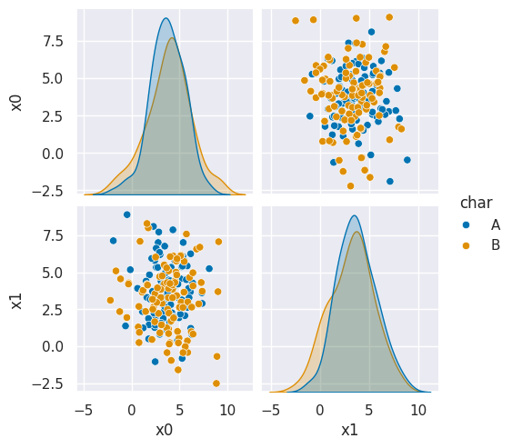
sns.pairplot(data=df6, hue='char', hue_order=['A','B'])
<seaborn.axisgrid.PairGrid at 0x7f7d4c91ce20>
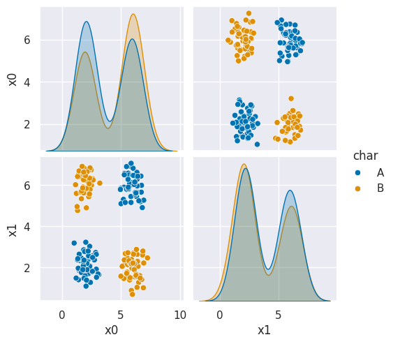
As we can see in this dataset, these classes are quite separated.
X_train, X_test, y_train, y_test = train_test_split(df6[['x0','x1']],df6['char'], random_state=4)
gnb_corners = GaussianNB()
gnb_corners.fit(X_train,y_train)
gnb_corners.score(X_test, y_test)
0.72
But we do not get a very good classification score.
To see why, we can look at what it learned.
N = 100
gnb_df = pd.DataFrame(np.concatenate([np.random.multivariate_normal(th, sig*np.eye(2),N)
         for th, sig in zip(gnb_corners.theta_,gnb_corners.var_)]),
         columns = ['x0','x1'])
gnb_df['char'] = [ci for cl in [[c]*N for c in gnb_corners.classes_] for ci in cl]

sns.pairplot(data =gnb_df, hue='char',hue_order=['A','B'])
<seaborn.axisgrid.PairGrid at 0x7f7d54699b20>
df6_pred = X_test.copy()
df6_pred['pred'] = gnb_corners.predict(X_test)
sns.pairplot(data =df6_pred, hue ='pred', hue_order =['A','B'])
<seaborn.axisgrid.PairGrid at 0x7f7d49ee0910>
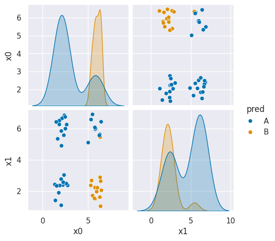
This does not look much like the data and it’s hard to tell which is higher at any given point in the 2D space. We know though, that it has missed the mark. We can also look at the actual predictions.
If you try this again, split, fit, plot, it will learn different decisions, but always at least about 25% of the data will have to be classified incorrectly.
12.3.1. Decision Trees#
This data does not fit the assumptions of the Niave Bayes model, but a decision tree has a different rule. It can be more complex, but for the scikit learn one relies on splitting the data at a series of points along one axis at a time.
It is a discriminative model, because it describes how to discriminate (in the sense of differentiate) between the classes. This is in contrast to the generative model that describes how the data is distributed.
dt = tree.DecisionTreeClassifier()
dt.fit(X_train,y_train)
DecisionTreeClassifier()In a Jupyter environment, please rerun this cell to show the HTML representation or trust the notebook.
On GitHub, the HTML representation is unable to render, please try loading this page with nbviewer.org.
DecisionTreeClassifier()
dt.score(X_test,y_test)
1.0
The sklearn estimator objects (that corresond to different models) all have the same API, so the fit, predict, and score methods are the same as above. We will see this also in regression and clustering. What each method does in terms of the specific calculations will vary depending on the model, but they’re always there.
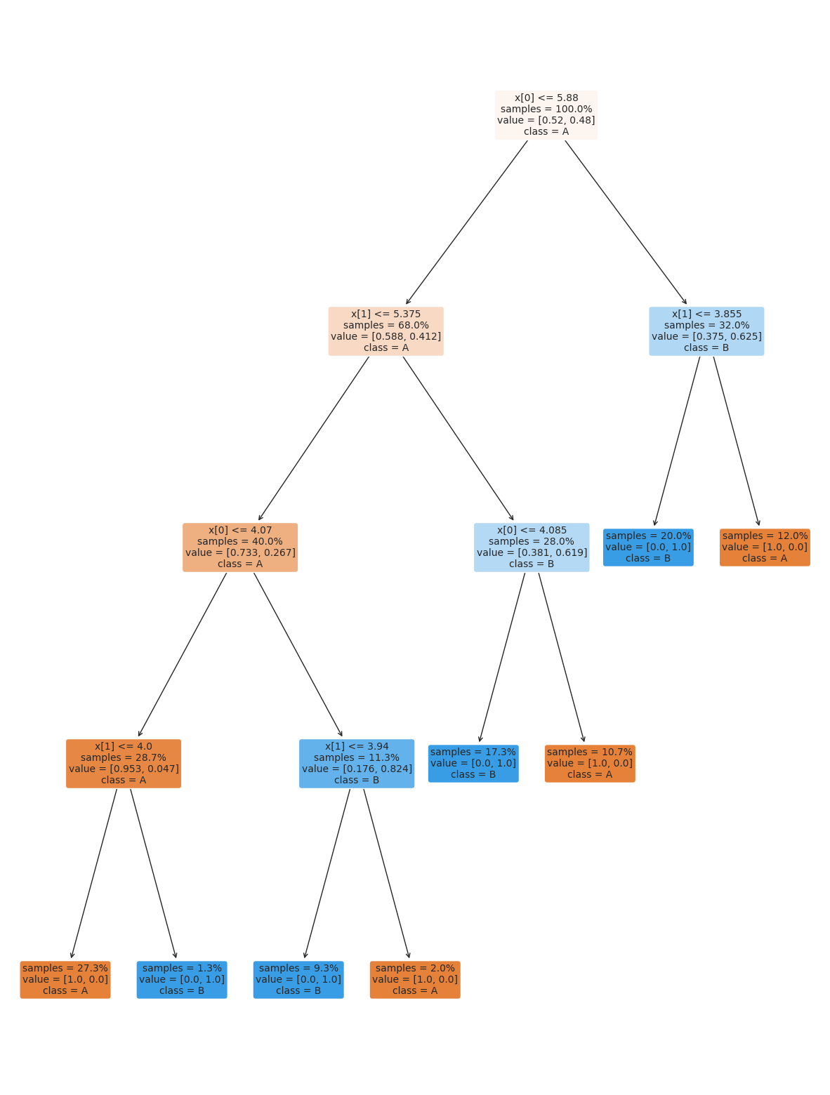
the tree module also allows you to plot the tree to examine it.
plt.figure(figsize=(15,20))
tree.plot_tree(dt, rounded =True, class_names = ['A','B'],
      proportion=True, filled =True, impurity=False,fontsize=10);
On the iris dataset, the sklearn docs include a diagram showing the decision boundary You should be able to modify this for another classifier.
12.4. Setting Classifier Parameters#
The decision tree we had above has a lot more layers than we would expect. This is really simple data so we still got perfect classification. However, the more complex the model, the more risk that it will learn something noisy about the training data that doesn’t hold up in the test set.
Fortunately, we can control the parameters to make it find a simpler decision boundary.
dt2 = tree.DecisionTreeClassifier(max_depth=2)
dt2.fit(X_train,y_train)
dt2.score(X_test,y_test)
plt.figure(figsize=(15,20))
tree.plot_tree(dt2, rounded =True, class_names = ['A','B'],
      proportion=True, filled =True, impurity=False,fontsize=10);
We can compute other metrics from the confusion matrix:
12.5. Questions After Class#
12.5.1. When should you start focusing on portfolio check 2?#
When you get P1 feedback
12.5.2. when will p1 check be graded?#
As soon as possible.
12.5.3. why not use a decision tree initially for the iris dataset?#
To teach the Gaussian Naive Bayes classifier, because learning different types of classifiers helps you understand the concept better.
12.5.4. Are there any popular machine learning models that use decision trees?#
Yes, a lot of medical appilcations do, because since they are easy to understand, it is easier for healthcare providers to trust them.
12.5.5. Do predictive algorithms have pros and cons? Or is there a standard?#
Each algorithm has different properties and strengths and weaknesses. Some are more popular than others, but they all do have weaknesses.
12.5.6. Different kinds of trees/charts, analyze what they mean and how to translate those#
12.5.7. is it possible after training the model to add more data to it ?#
The models we will see in class, no. However, there is a thing called “online learning” that involves getting more data on a regular basis to improve its performance.