14. Clustering Metrics#
14.1. Comparing Classification and Clustering Data#
Datasets for classification must have a target variable observed, but we can drop it to use it for clustering
14.2. KMeans review#
clustering goal: find groups of samples that are similar
k-means assumption: a fixed number (\(k\)) of means will describe the data enough to find the groups
14.3. Clustering with Sci-kit Learn#
import seaborn as sns
import numpy as np
import matplotlib.pylab as plt
from sklearn import datasets
from sklearn.cluster import KMeans
from sklearn import metrics
import pandas as pd
sns.set_theme(palette='colorblind')

# set global random seed so that the notes are the same each time the site builds
np.random.seed(1103)
Today we will load the iris data from seaborn:
iris_df = sns.load_dataset('iris')
iris_df.head()
| sepal_length | sepal_width | petal_length | petal_width | species | |
|---|---|---|---|---|---|
| 0 | 5.1 | 3.5 | 1.4 | 0.2 | setosa |
| 1 | 4.9 | 3.0 | 1.4 | 0.2 | setosa |
| 2 | 4.7 | 3.2 | 1.3 | 0.2 | setosa |
| 3 | 4.6 | 3.1 | 1.5 | 0.2 | setosa |
| 4 | 5.0 | 3.6 | 1.4 | 0.2 | setosa |
Remember this is how the clustering algorithm sees the data, with no labels:
sns.pairplot(iris_df)
<seaborn.axisgrid.PairGrid at 0x7f4411ea8310>
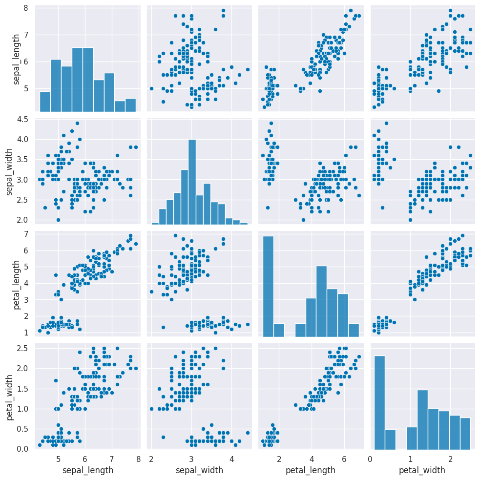
Next we need to create a copy of the data that’s appropriate for clustering. Remember that clustering is unsupervised so it doesn’t have a target variable. We also can do clustering on the data with or without splitting into test/train splits, since it doesn’t use a target variable, we can evaluate how good the clusters it finds are on the actual data that it learned from.
We can either pick the measurements out or drop the species column. remember most data frame operations return a copy of the dataframe.
iris_X = iris_df.drop(columns=['species'])
iris_X.head()
| sepal_length | sepal_width | petal_length | petal_width | |
|---|---|---|---|---|
| 0 | 5.1 | 3.5 | 1.4 | 0.2 |
| 1 | 4.9 | 3.0 | 1.4 | 0.2 |
| 2 | 4.7 | 3.2 | 1.3 | 0.2 |
| 3 | 4.6 | 3.1 | 1.5 | 0.2 |
| 4 | 5.0 | 3.6 | 1.4 | 0.2 |
Next, we create a Kmeans estimator object with 3 clusters, since we know that the iris data has 3 species of flowers. We refer to these three groups as classes in classification (the goal is to label the classes…) and in clustering we sometimes borrow that word. Sometimes, clustering literature will be more abstract and refer to partitions, this is especially common in more mathematical/statistical work as opposed to algorithmic work on clustering.
km = KMeans(n_clusters=3)
We dropped the column that tells us which of the three classes that each sample(row) belongs to. We still have data from three species of flows.
Hint
use shift+tab or another jupyter help to figure out what the parameter names are for any function or class you’re working with.
Since we don’t have separate test and train data, we can use the fit_predict method. This is what the kmeans algorithm always does anyway, it both learns the means and the assignment (or prediction) for each sample at the same time.
km.fit_predict(iris_X)
/opt/hostedtoolcache/Python/3.8.18/x64/lib/python3.8/site-packages/sklearn/cluster/_kmeans.py:1416: FutureWarning: The default value of `n_init` will change from 10 to 'auto' in 1.4. Set the value of `n_init` explicitly to suppress the warning
  super()._check_params_vs_input(X, default_n_init=10)
array([0, 0, 0, 0, 0, 0, 0, 0, 0, 0, 0, 0, 0, 0, 0, 0, 0, 0, 0, 0, 0, 0,
       0, 0, 0, 0, 0, 0, 0, 0, 0, 0, 0, 0, 0, 0, 0, 0, 0, 0, 0, 0, 0, 0,
       0, 0, 0, 0, 0, 0, 1, 1, 2, 1, 1, 1, 1, 1, 1, 1, 1, 1, 1, 1, 1, 1,
       1, 1, 1, 1, 1, 1, 1, 1, 1, 1, 1, 2, 1, 1, 1, 1, 1, 1, 1, 1, 1, 1,
       1, 1, 1, 1, 1, 1, 1, 1, 1, 1, 1, 1, 2, 1, 2, 2, 2, 2, 1, 2, 2, 2,
       2, 2, 2, 1, 1, 2, 2, 2, 2, 1, 2, 1, 2, 1, 2, 2, 1, 1, 2, 2, 2, 2,
       2, 1, 2, 2, 2, 2, 1, 2, 2, 2, 1, 2, 2, 2, 1, 2, 2, 1], dtype=int32)
This gives the labeled cluster by index, or the assignment, of each point.
If we run that a few times, we will see different solutions each time because the algorithm is random, or stochastic.
These are similar to the outputs in classification, except that in classification, it’s able to tell us a specific species for each. Here it can only say clust 0, 1, or 2. It can’t match those groups to the species of flower.
Now that we know what these are, we can save them to our DataFrame
iris_df['km3_1'] = km.fit_predict(iris_X)
/opt/hostedtoolcache/Python/3.8.18/x64/lib/python3.8/site-packages/sklearn/cluster/_kmeans.py:1416: FutureWarning: The default value of `n_init` will change from 10 to 'auto' in 1.4. Set the value of `n_init` explicitly to suppress the warning
  super()._check_params_vs_input(X, default_n_init=10)
14.4. Visualizing the outputs#
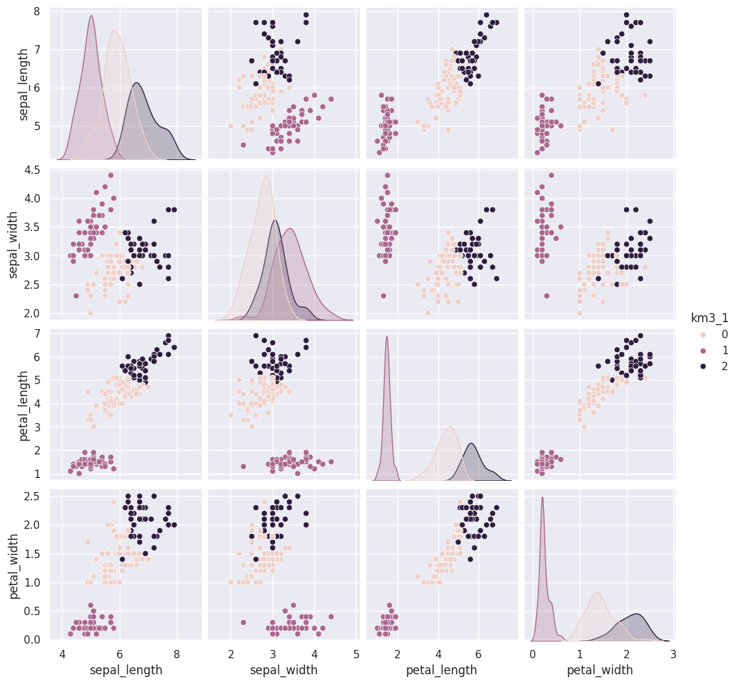
Add the predictions as a new column to the original iris_df and make a pairplot with the points colored by what the clustering learned.
sns.pairplot(data=iris_df,hue='km3_1')
<seaborn.axisgrid.PairGrid at 0x7f440e7d7160>
14.5. Clustering Persistence#
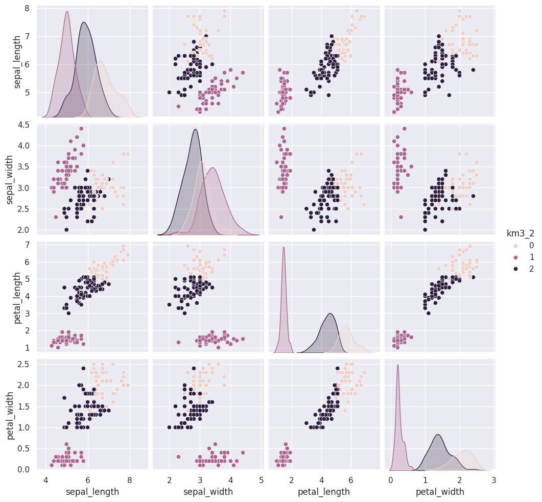
We can run kmeans a few more times and plot each time and/or compare with a neighbor/ another group.
iris_df['km3_2'] = km.fit_predict(iris_X)
/opt/hostedtoolcache/Python/3.8.18/x64/lib/python3.8/site-packages/sklearn/cluster/_kmeans.py:1416: FutureWarning: The default value of `n_init` will change from 10 to 'auto' in 1.4. Set the value of `n_init` explicitly to suppress the warning
  super()._check_params_vs_input(X, default_n_init=10)
We can use the vars parameter to plot only the measurement columns and not the cluster labels. We didn’t have to do this before, because species is strings, so seaborn knows to not plot it, but the cluster predictions are also numerical, so by default seaborn plots them.
measurement_cols = ['sepal_length', 'sepal_width', 'petal_length', 'petal_width']
sns.pairplot(data=iris_df,hue = 'km3_2', vars=measurement_cols)
<seaborn.axisgrid.PairGrid at 0x7f440ef75340>
iris_df['km3_3'] = km.fit_predict(iris_X)
measurement_cols = ['sepal_length', 'sepal_width', 'petal_length', 'petal_width']
sns.pairplot(data=iris_df,hue = 'km3_3', vars=measurement_cols)
/opt/hostedtoolcache/Python/3.8.18/x64/lib/python3.8/site-packages/sklearn/cluster/_kmeans.py:1416: FutureWarning: The default value of `n_init` will change from 10 to 'auto' in 1.4. Set the value of `n_init` explicitly to suppress the warning
  super()._check_params_vs_input(X, default_n_init=10)
<seaborn.axisgrid.PairGrid at 0x7f4403f79f70>

We will use a loop to add a few more.
for i in range(4,15):
    iris_df['km3_' +str(i)] = km.fit_predict(iris_X)
/opt/hostedtoolcache/Python/3.8.18/x64/lib/python3.8/site-packages/sklearn/cluster/_kmeans.py:1416: FutureWarning: The default value of `n_init` will change from 10 to 'auto' in 1.4. Set the value of `n_init` explicitly to suppress the warning
  super()._check_params_vs_input(X, default_n_init=10)
/opt/hostedtoolcache/Python/3.8.18/x64/lib/python3.8/site-packages/sklearn/cluster/_kmeans.py:1416: FutureWarning: The default value of `n_init` will change from 10 to 'auto' in 1.4. Set the value of `n_init` explicitly to suppress the warning
  super()._check_params_vs_input(X, default_n_init=10)
/opt/hostedtoolcache/Python/3.8.18/x64/lib/python3.8/site-packages/sklearn/cluster/_kmeans.py:1416: FutureWarning: The default value of `n_init` will change from 10 to 'auto' in 1.4. Set the value of `n_init` explicitly to suppress the warning
  super()._check_params_vs_input(X, default_n_init=10)
/opt/hostedtoolcache/Python/3.8.18/x64/lib/python3.8/site-packages/sklearn/cluster/_kmeans.py:1416: FutureWarning: The default value of `n_init` will change from 10 to 'auto' in 1.4. Set the value of `n_init` explicitly to suppress the warning
  super()._check_params_vs_input(X, default_n_init=10)
/opt/hostedtoolcache/Python/3.8.18/x64/lib/python3.8/site-packages/sklearn/cluster/_kmeans.py:1416: FutureWarning: The default value of `n_init` will change from 10 to 'auto' in 1.4. Set the value of `n_init` explicitly to suppress the warning
  super()._check_params_vs_input(X, default_n_init=10)
/opt/hostedtoolcache/Python/3.8.18/x64/lib/python3.8/site-packages/sklearn/cluster/_kmeans.py:1416: FutureWarning: The default value of `n_init` will change from 10 to 'auto' in 1.4. Set the value of `n_init` explicitly to suppress the warning
  super()._check_params_vs_input(X, default_n_init=10)
/opt/hostedtoolcache/Python/3.8.18/x64/lib/python3.8/site-packages/sklearn/cluster/_kmeans.py:1416: FutureWarning: The default value of `n_init` will change from 10 to 'auto' in 1.4. Set the value of `n_init` explicitly to suppress the warning
  super()._check_params_vs_input(X, default_n_init=10)
/opt/hostedtoolcache/Python/3.8.18/x64/lib/python3.8/site-packages/sklearn/cluster/_kmeans.py:1416: FutureWarning: The default value of `n_init` will change from 10 to 'auto' in 1.4. Set the value of `n_init` explicitly to suppress the warning
  super()._check_params_vs_input(X, default_n_init=10)
/opt/hostedtoolcache/Python/3.8.18/x64/lib/python3.8/site-packages/sklearn/cluster/_kmeans.py:1416: FutureWarning: The default value of `n_init` will change from 10 to 'auto' in 1.4. Set the value of `n_init` explicitly to suppress the warning
  super()._check_params_vs_input(X, default_n_init=10)
/opt/hostedtoolcache/Python/3.8.18/x64/lib/python3.8/site-packages/sklearn/cluster/_kmeans.py:1416: FutureWarning: The default value of `n_init` will change from 10 to 'auto' in 1.4. Set the value of `n_init` explicitly to suppress the warning
  super()._check_params_vs_input(X, default_n_init=10)
/opt/hostedtoolcache/Python/3.8.18/x64/lib/python3.8/site-packages/sklearn/cluster/_kmeans.py:1416: FutureWarning: The default value of `n_init` will change from 10 to 'auto' in 1.4. Set the value of `n_init` explicitly to suppress the warning
  super()._check_params_vs_input(X, default_n_init=10)
If we look at the assignments, we can see how similar they are.
iris_df[measurement_cols].sample(10)
| sepal_length | sepal_width | petal_length | petal_width | |
|---|---|---|---|---|
| 90 | 5.5 | 2.6 | 4.4 | 1.2 |
| 21 | 5.1 | 3.7 | 1.5 | 0.4 |
| 80 | 5.5 | 2.4 | 3.8 | 1.1 |
| 62 | 6.0 | 2.2 | 4.0 | 1.0 |
| 114 | 5.8 | 2.8 | 5.1 | 2.4 |
| 19 | 5.1 | 3.8 | 1.5 | 0.3 |
| 13 | 4.3 | 3.0 | 1.1 | 0.1 |
| 41 | 4.5 | 2.3 | 1.3 | 0.3 |
| 69 | 5.6 | 2.5 | 3.9 | 1.1 |
| 95 | 5.7 | 3.0 | 4.2 | 1.2 |
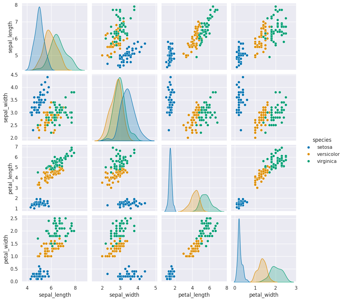
Notice that while the numbers vary across the columns, the same rows have are the same or different across the columns. This means that each sample sometimes gets assigned to a different label, but the same ones are grouped together.
sns.pairplot(iris_df,hue='species',vars=measurement_cols)
<seaborn.axisgrid.PairGrid at 0x7f4444990820>
iris_df.columns
Index(['sepal_length', 'sepal_width', 'petal_length', 'petal_width', 'species',
       'km3_1', 'km3_2', 'km3_3', 'km3_4', 'km3_5', 'km3_6', 'km3_7', 'km3_8',
       'km3_9', 'km3_10', 'km3_11', 'km3_12', 'km3_13', 'km3_14'],
      dtype='object')
The grouping of the points stay the same across different runs, but which color each group gets assigned to changes. Which blob is which color changes, but the partitions are basically the same.
Today, we saw that the clustering solution was pretty similar each time in terms of which points were grouped together, but the labeling of the groups (which one was each number) was different each time. We also saw that clustering can only number the clusters, it can’t match them with certainty to the species. This makes evaluating clustering somewhat different, so we need new metrics.
14.6. Clustering Evaluation#
a: The mean distance between a sample and all other points in the same class.
b: The mean distance between a sample and all other points in the next nearest cluster.
This score computes a ratio of how close points are to points in the same cluster vs other clusters
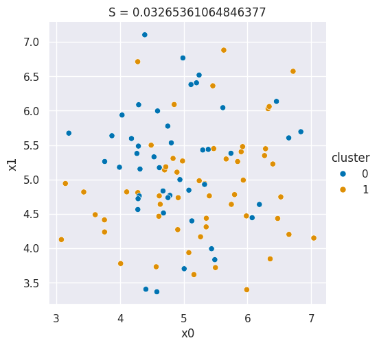
We drew pictures in prismia, but we can also generate samples to make a plot that shows a bad silhouette score:
Show code cell source
N = 100
bad_cluster_data = np.random.multivariate_normal([5,5],.75*np.eye(2), size=N)
data_cols = ['x0','x1']
df = pd.DataFrame(data=bad_cluster_data,columns=data_cols)
df['cluster'] = np.random.choice([0,1],N)

sns.relplot(data=df,x='x0',y='x1',hue='cluster',)
plt.title('S = ' + str(metrics.silhouette_score(df[data_cols],df['cluster'])));
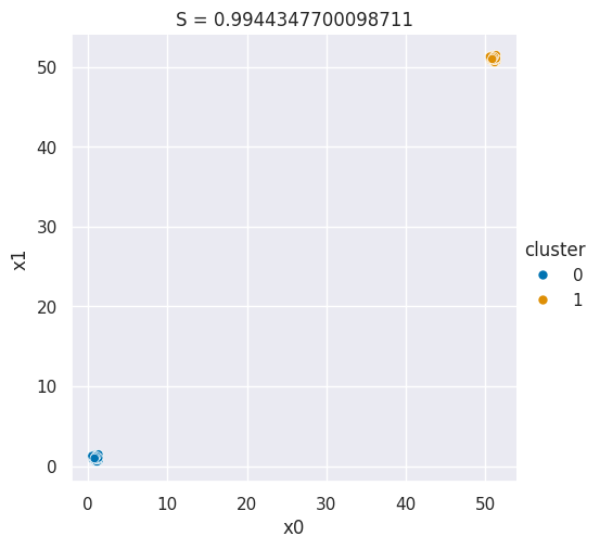
And we can make a plot for a good silhouette score
Show code cell source
N = 50
single_cluster = np.random.multivariate_normal([1,1],
                                                .05*np.eye(2),
                                                 size=N)
good_cluster_data = np.concatenate([single_cluster,50+single_cluster])
data_cols = ['x0','x1']
df = pd.DataFrame(data=good_cluster_data,columns=data_cols)
df['cluster'] = [0]*N + [1]*N

sns.relplot(data=df,x='x0',y='x1',hue='cluster',)
plt.title('S = ' + str(metrics.silhouette_score(df[data_cols],df['cluster'])));
Then we can use the silhouette score on our existing clustering solutions.
metrics.silhouette_score(iris_X,iris_df['km3_2'])
0.5528190123564102
We can also apply it using a lambda:
sil = lambda col: metrics.silhouette_score(iris_X, col)
iris_df[['km3_1', 'km3_2', 'km3_3', 'km3_4', 'km3_5', 'km3_6', 'km3_7', 'km3_8',
       'km3_9', 'km3_10', 'km3_11', 'km3_12', 'km3_13', 'km3_14']].apply(sil)
km3_1     0.552819
km3_2     0.552819
km3_3     0.552819
km3_4     0.552819
km3_5     0.552819
km3_6     0.552819
km3_7     0.552819
km3_8     0.552819
km3_9     0.552819
km3_10    0.552819
km3_11    0.552819
km3_12    0.552819
km3_13    0.552819
km3_14    0.552819
dtype: float64
All of these solutions were the same
14.7. Finding the right number of Clusters#
When we do not know the right number, we can try different numbers and compare the silhouette score.
km2 = KMeans(n_clusters=2)
iris_df['km2'] = km2.fit_predict(iris_X)

km4 = KMeans(n_clusters=4)
iris_df['km4'] = km4.fit_predict(iris_X)
metrics.silhouette_score(iris_df[measurement_cols],iris_df['km2']), metrics.silhouette_score(iris_df[measurement_cols],iris_df['km4'])
/opt/hostedtoolcache/Python/3.8.18/x64/lib/python3.8/site-packages/sklearn/cluster/_kmeans.py:1416: FutureWarning: The default value of `n_init` will change from 10 to 'auto' in 1.4. Set the value of `n_init` explicitly to suppress the warning
  super()._check_params_vs_input(X, default_n_init=10)
/opt/hostedtoolcache/Python/3.8.18/x64/lib/python3.8/site-packages/sklearn/cluster/_kmeans.py:1416: FutureWarning: The default value of `n_init` will change from 10 to 'auto' in 1.4. Set the value of `n_init` explicitly to suppress the warning
  super()._check_params_vs_input(X, default_n_init=10)
(0.6810461692117465, 0.49805050499728815)
For this datast, 2 clusters describes the data best, even though the dat came from 3 species of flowers. This is a common thing to observe.
While we sometims describe things as discrete, in nature a lot of things vary fairly continuously. Clustering works best for things that are truly discrete, but can be useful even when it is not a perfct fit.
14.8. Mutual Information#
When we know the truth, we can see if the learned clusters are related to the true groups, we can’t compare them like accuracy but we can use a metric that is intuitively like a correlation for categorical variables, the mutual information.
The adjusted_mutual_info_score method in the metrics module computes a version of mutual information that is normalized to have good properties.
metrics.adjusted_mutual_info_score(iris_df['species'],iris_df['km3_1'])
0.7551191675800485
metrics.adjusted_mutual_info_score(iris_df['species'],iris_df['km3_2'])
0.7551191675800484
14.9. Questions After Class#
14.9.1. How do you know the right number of clusters to use before knowing anything about the data?#
You do not. You have to try it out. Either like we did above by trying different numbers and checking the score, or using a clustering technique that can learn the number at the same time.
14.9.2. How to determine which cluster is what?#
That you have to assign based on looking at the samples. Remember in a real clustering situation, you do not know what the groups are.
Typically, once we find the clusters, we look at the a few samples in each cluster to try to assign a name for it. For example in th Etsy case of clustering product images to find “styles” after they have the groups of images, they look at a few that are near the “center” of the cluster for each cluster to come up with a name for each one.
In the COPD example, after they found the groups, the doctors continued studying what was going on in each group. They will do genetic analysis and continue studying to try to decide a name for each.
14.9.3. Difference between k-means, elbow, and silhouette#
K-means is the clustering algorithm. The elbow technique refers to plotting the score for different solutions and then picking the one at that looks like an elbow or right before it to be your final thing. Silhoette is a score to evaluate clustering solutions.
