6. Tidy Data and Structural Repairs

6.1. Intro

This week, we’ll be cleaning data.

Cleaning data is labor intensive and requires making subjective choices.
We’ll focus on, and assess you on, manipulating data correctly, making reasonable choices, and documenting the choices you make carefully.

We’ll focus on the programming tools that get used in cleaning data in class this week:

• reshaping data

• handling missing or incorrect values

• renaming columns

Warning

this is incomplete, but will get filled in this week.

import pandas as pd
import seaborn as sns

# make plots look nicer and increase font size
sns.set_theme(font_scale=2, palette='colorblind')

6.2. What is Tidy Data

Read in the three csv files described below and store them in a list of dataFrames

url_base = 'https://raw.githubusercontent.com/rhodyprog4ds/rhodyds/main/data/'

datasets = ['study_a.csv','study_b.csv','study_c.csv']

study_df_list = [pd.read_csv(url_base +cur_study,na_values='-') 
                 for cur_study in datasets]

study_df_list[0]

	name	treatmenta	treatmentb
0	John Smith	NaN	2
1	Jane Doe	16.0	11
2	Mary Johnson	3.0	1

study_df_list[1]

	intervention	John Smith	Jane Doe	Mary Johnson
0	treatmenta	NaN	16	3
1	treatmentb	2.0	11	1

study_df_list[2]

	person	treatment	result
0	John Smith	a	NaN
1	Jane Doe	a	16.0
2	Mary Johnson	a	3.0
3	John Smith	b	2.0
4	Jane Doe	b	11.0
5	Mary Johnson	b	1.0

These three all show the same data, but let’s say we have two goals:

• find the average effect per person across treatments

• find the average effect per treatment across people

This works differently for these three versions.

df_a = study_df_list[0]
df_a.mean(numeric_only=True,)

treatmenta    9.500000
treatmentb    4.666667
dtype: float64

we get the average per treatment, but to get the average per person, we have to go across rows, which we can do here, but doesn’t work as well with plotting

we can work across rows with the axis parameter if needed

df_a.mean(numeric_only=True,axis=1)

0     2.0
1    13.5
2     2.0
dtype: float64

df_b = study_df_list[1]
df_b

	intervention	John Smith	Jane Doe	Mary Johnson
0	treatmenta	NaN	16	3
1	treatmentb	2.0	11	1

Now we get the average per person, but what about per treatment? again we have to go across rows instead.

study_df_list[2]

	person	treatment	result
0	John Smith	a	NaN
1	Jane Doe	a	16.0
2	Mary Johnson	a	3.0
3	John Smith	b	2.0
4	Jane Doe	b	11.0
5	Mary Johnson	b	1.0

For the third one, however, we can use groupby, because this one is tidy.

study_df_list[2].groupby('treatment').mean(numeric_only=True)

	result
treatment
a	9.500000
b	4.666667

study_df_list[2].groupby('person').mean(numeric_only=True)

	result
person
Jane Doe	13.5
John Smith	2.0
Mary Johnson	2.0

The original Tidy Data paper is worth reading to build a deeper understanding of these ideas.

6.3. Tidying Data

Let’s reshape the first one to match the tidy one. First, we will save it to a DataFrame, this makes things easier to read and enables us to use the built in help in jupyter, because it can’t check types too many levels into a data structure.

df_a.melt(id_vars='name', value_vars=['treatmenta','treatmentb'])

	name	variable	value
0	John Smith	treatmenta	NaN
1	Jane Doe	treatmenta	16.0
2	Mary Johnson	treatmenta	3.0
3	John Smith	treatmentb	2.0
4	Jane Doe	treatmentb	11.0
5	Mary Johnson	treatmentb	1.0

When we melt a dataset:

• the id_vars stay as columns

• the data from the value_vars columns become the values in the value column

• the column names from the value_vars become the values in the variable column

• we can rename the value and the variable columns.

df_a.melt(id_vars='name', value_vars=['treatmenta','treatmentb'],
          var_name= 'treatment_type',
          value_name='result',)

	name	treatment_type	result
0	John Smith	treatmenta	NaN
1	Jane Doe	treatmenta	16.0
2	Mary Johnson	treatmenta	3.0
3	John Smith	treatmentb	2.0
4	Jane Doe	treatmentb	11.0
5	Mary Johnson	treatmentb	1.0

6.4. Transforming the Coffee Data

Let’s do it for our coffee data:

arabica_data_url = 'https://raw.githubusercontent.com/jldbc/coffee-quality-database/master/data/arabica_data_cleaned.csv'
# load the data
coffee_df = pd.read_csv(arabica_data_url, index_col=0)

coffee_df.head(2)

	Species	Owner	Country.of.Origin	Farm.Name	Lot.Number	Mill	ICO.Number	Company	Altitude	Region	...	Color	Category.Two.Defects	Expiration	Certification.Body	Certification.Address	Certification.Contact	unit_of_measurement	altitude_low_meters	altitude_high_meters	altitude_mean_meters
1	Arabica	metad plc	Ethiopia	metad plc	NaN	metad plc	2014/2015	metad agricultural developmet plc	1950-2200	guji-hambela	...	Green	0	April 3rd, 2016	METAD Agricultural Development plc	309fcf77415a3661ae83e027f7e5f05dad786e44	19fef5a731de2db57d16da10287413f5f99bc2dd	m	1950.0	2200.0	2075.0
2	Arabica	metad plc	Ethiopia	metad plc	NaN	metad plc	2014/2015	metad agricultural developmet plc	1950-2200	guji-hambela	...	Green	1	April 3rd, 2016	METAD Agricultural Development plc	309fcf77415a3661ae83e027f7e5f05dad786e44	19fef5a731de2db57d16da10287413f5f99bc2dd	m	1950.0	2200.0	2075.0

2 rows × 43 columns

coffee_df.columns

Index(['Species', 'Owner', 'Country.of.Origin', 'Farm.Name', 'Lot.Number',
       'Mill', 'ICO.Number', 'Company', 'Altitude', 'Region', 'Producer',
       'Number.of.Bags', 'Bag.Weight', 'In.Country.Partner', 'Harvest.Year',
       'Grading.Date', 'Owner.1', 'Variety', 'Processing.Method', 'Aroma',
       'Flavor', 'Aftertaste', 'Acidity', 'Body', 'Balance', 'Uniformity',
       'Clean.Cup', 'Sweetness', 'Cupper.Points', 'Total.Cup.Points',
       'Moisture', 'Category.One.Defects', 'Quakers', 'Color',
       'Category.Two.Defects', 'Expiration', 'Certification.Body',
       'Certification.Address', 'Certification.Contact', 'unit_of_measurement',
       'altitude_low_meters', 'altitude_high_meters', 'altitude_mean_meters'],
      dtype='object')

scores_of_interest = ['Aroma',
       'Flavor', 'Aftertaste', 'Acidity', 'Body', 'Balance', 'Uniformity',
       'Clean.Cup', 'Sweetness',]

coffee_df[scores_of_interest].head(2)

	Aroma	Flavor	Aftertaste	Acidity	Body	Balance	Uniformity	Clean.Cup	Sweetness
1	8.67	8.83	8.67	8.75	8.50	8.42	10.0	10.0	10.0
2	8.75	8.67	8.50	8.58	8.42	8.42	10.0	10.0	10.0

We can make this tall using melt to transform with that set of questions and then rename the value and variable columns to be descriptive.

coffee_df_tall = coffee_df.melt(id_vars='Country.of.Origin',value_vars=scores_of_interest,
               var_name='rating_type',
               value_name='score')
coffee_df_tall.head(1)

	Country.of.Origin	rating_type	score
0	Ethiopia	Aroma	8.67

Notice that the actual column names inside the scores_of_interest variable become the values in the variable column.

This one we can plot in more ways:

sns.displot(data = coffee_df_tall, kind = 'kde', x='score',
            col='rating_type', hue='Country.of.Origin',col_wrap=3)

/tmp/ipykernel_2149/2608901824.py:1: UserWarning: Dataset has 0 variance; skipping density estimate. Pass `warn_singular=False` to disable this warning.
  sns.displot(data = coffee_df_tall, kind = 'kde', x='score',

<seaborn.axisgrid.FacetGrid at 0x7f23c4c3fc10>

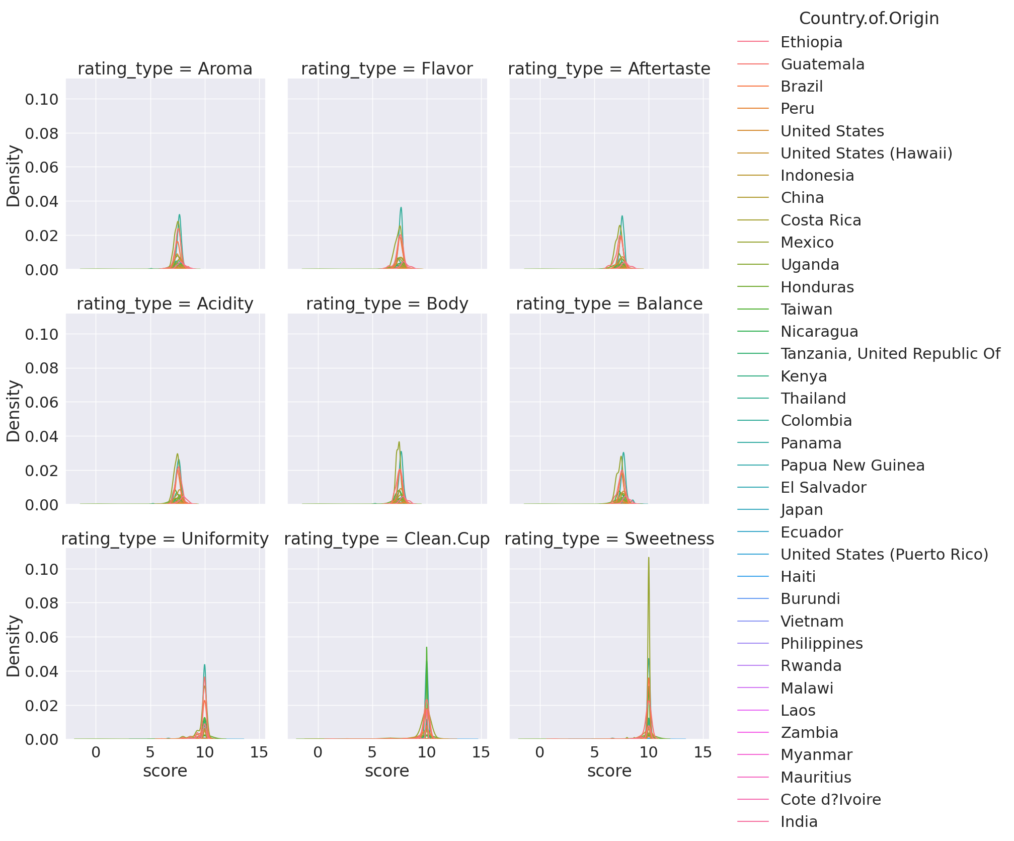
find why warning

6.5. Filtering Data

Warning

this was not in class this week, but is added here for completeness

high_prod = coffee_df[coffee_df['Number.of.Bags']>250]
high_prod.shape

(368, 43)

coffee_df.shape

(1311, 43)

We see that filters and reduces. We can use any boolean expression in the square brackets.

top_balance = coffee_df[coffee_df['Balance']>coffee_df['Balance'].quantile(.75)]
top_balance.shape

(252, 43)

We can confirm that we got only the top 25% of balance scores:

top_balance.describe()

	Number.of.Bags	Aroma	Flavor	Aftertaste	Acidity	Body	Balance	Uniformity	Clean.Cup	Sweetness	Cupper.Points	Total.Cup.Points	Moisture	Category.One.Defects	Quakers	Category.Two.Defects	altitude_low_meters	altitude_high_meters	altitude_mean_meters
count	252.000000	252.000000	252.000000	252.000000	252.000000	252.000000	252.000000	252.000000	252.000000	252.000000	252.000000	252.00000	252.000000	252.000000	252.000000	252.000000	190.000000	190.000000	190.000000
mean	153.337302	7.808889	7.837659	7.734167	7.824881	7.780159	8.003095	9.885278	9.896667	9.885952	7.865714	84.52504	0.072579	0.361111	0.150794	2.801587	1343.138168	1424.547053	1383.842611
std	126.498576	0.355319	0.318172	0.302481	0.320253	0.317712	0.213056	0.363303	0.470514	0.380433	0.383738	1.91563	0.051682	1.249923	0.692216	4.659771	480.927004	503.063351	484.286247
min	0.000000	5.080000	7.170000	6.920000	7.080000	5.250000	7.830000	6.670000	5.330000	6.670000	5.170000	77.00000	0.000000	0.000000	0.000000	0.000000	1.000000	1.000000	1.000000
25%	12.750000	7.647500	7.670000	7.500000	7.670000	7.670000	7.830000	10.000000	10.000000	10.000000	7.670000	83.42000	0.000000	0.000000	0.000000	0.000000	1162.500000	1200.000000	1200.000000
50%	165.500000	7.780000	7.830000	7.750000	7.830000	7.750000	7.920000	10.000000	10.000000	10.000000	7.830000	84.46000	0.100000	0.000000	0.000000	1.000000	1400.000000	1500.000000	1450.000000
75%	275.000000	8.000000	8.000000	7.920000	8.000000	7.920000	8.080000	10.000000	10.000000	10.000000	8.080000	85.52000	0.110000	0.000000	0.000000	3.000000	1695.000000	1800.000000	1750.000000
max	360.000000	8.750000	8.830000	8.670000	8.750000	8.580000	8.750000	10.000000	10.000000	10.000000	9.250000	90.58000	0.210000	10.000000	6.000000	40.000000	2560.000000	2560.000000	2560.000000

We can also use the isin method to filter by comparing to an iterable type

total_per_country = coffee_df.groupby('Country.of.Origin')['Number.of.Bags'].sum()
top_countries = total_per_country.sort_values(ascending=False)[:10].index
top_coffee_df = coffee_df[coffee_df['Country.of.Origin'].isin(top_countries)]

6.6. More manipulations

Warning

this was not in class this week, but is added here for completeness

Here, we will make a tiny DataFrame from scratch to illustrate a couple of points

large_num_df = pd.DataFrame(data= [[730000000,392000000,580200000],
                                   [315040009,580000000,967290000]],
                           columns = ['a','b','c'])
large_num_df

	a	b	c
0	730000000	392000000	580200000
1	315040009	580000000	967290000

This dataet is not tidy, but making it this way was faster to set it up. We could make it tidy using melt as is.

large_num_df.melt()

	variable	value
0	a	730000000
1	a	315040009
2	b	392000000
3	b	580000000
4	c	580200000
5	c	967290000

However, I want an additional variable, so I wil reset the index, which adds an index column for the original index and adds a new index that is numerical. In this case they’re the same.

large_num_df.reset_index()

	index	a	b	c
0	0	730000000	392000000	580200000
1	1	315040009	580000000	967290000

If I melt this one, using the index as the id, then I get a reasonable tidy DataFrame

ls_tall_df = large_num_df.reset_index().melt(id_vars='index')
ls_tall_df

	index	variable	value
0	0	a	730000000
1	1	a	315040009
2	0	b	392000000
3	1	b	580000000
4	0	c	580200000
5	1	c	967290000

Now, we can plot.

sns.catplot(data = ls_tall_df,x='variable',y='value',
            hue='index',kind='bar')

<seaborn.axisgrid.FacetGrid at 0x7f23bf8dde80>

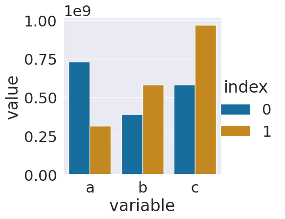
Since the numbers are so big, this might be hard to interpret. Displaying it with all the 0s would not be easier to read. The best thing to do is to add a new colum with adjusted values and a corresponding title.

ls_tall_df['value (millions)'] = ls_tall_df['value']/1000000
ls_tall_df.head()

	index	variable	value	value (millions)
0	0	a	730000000	730.000000
1	1	a	315040009	315.040009
2	0	b	392000000	392.000000
3	1	b	580000000	580.000000
4	0	c	580200000	580.200000

Now we can plot again, with the smaller values and an updated axis label. Adding a column with the adjusted title is good practice because it does not lose any data and since we set the value and the title at the same time it keeps it clear what the values are.

6.7. Questions after Class

6.7.1. In the data we had about treatment a and treatment b. Say there was another column that provided information about the age of the people. Could we create another value variable to or would we put it in the value_vars list along with treatment a and treatmentb?

We can have multiple variables as the id_vars so that the dataset would have 4 columns instead of 3.

6.7.2. Are there any prebuilt methods to identify and remove extreme outliers?

There may be, that is a good thing to look in the documentation for. However, typically the definition of an outlier is best made within context, so the filtering strategy that we just used would be the way to remove them, after doign some EDA.

6.7.3. Is there a specific metric to which a dataset must meet to consider it ‘cleaned’?

It’s “clean” when it will work for the analysis you want to do. This means clean enough for one analysis may not be enough for another goal. Domain expertise is alwasy important.

6.7.4. how does melt work underneath the hood?

The melt documentation is the place to read about the details. It also includes alink to the source code if reading how it is implemented in code is more helpful to you can reading English.

6.7.5. Do people ever write their melted datasets to new files for redistribution, maybe to make things easier for future researchers?

Yes! If you look in the R Tidy Tuesday datsets most distribute the “raw” and cleaned data.

6.7.6. the ending graphs are hard to read. Is there a way to label specific countries kde lines?

Yes

6.7.7. how do you get the index of something in a row

I do not understand this question, please reach out with more info so that I can help you

6.7.8. i was trying to do somthing earlier where I got the max of a column but wanted to know somthing else associated with that row

most pandas methods allow you to use axis to apply them across rows instead of columns

6.7.9. cleaning out different data types

Once the data is loaded into pandas, we can use all of the same techniques

6.7.10. Is there a scenario where a dataset cannot be cleaned using pandas methods?

yes, there are cases where cleaning the already loaded dataframe is not the best way to make the necessary fixes. One tool that can help is called Openrefine it is an open source program that provides a GUI based interface to clean data, but also outputs a script of what actions were taking, to make the cleaning replicable.

This is something you could learn about and try for the level 3 prepare achievement in your portfolio. One resource for learning it is the Data Carpentry lesson on Data Cleaning for Ecologists

6.7.11. Is there another standard format for sharing cleaned datasets?

.csv is the widely accepted preferred format for well strucutured tabular data that is of reasonable size. If it is too large, a database might (next week!) can be useful.

6.7.12. With extremely large datasets, is there a way to find what pieces of the dataset are missing values other than manually checking

Using strategies like we did to day, by testing dropping and the EDA strategies that we used last week can help. If it is a very large dataset, you may need to use more powerful system, but the basics work out the same.

Also, remember in most contexts, you will have some relevant domain knowledge that can help you.