16. Interpretting Regression

import numpy as np
import seaborn as sns
import matplotlib.pyplot as plt
from sklearn import datasets, linear_model
from sklearn.metrics import mean_squared_error, r2_score
from sklearn.model_selection import train_test_split
import pandas as pd
sns.set_theme(font_scale=2,palette='colorblind')

16.1. Review - Univariate regression

(see previous class notes here)

tips_df = sns.load_dataset('tips')
tips_df.head()

	total_bill	tip	sex	smoker	day	time	size
0	16.99	1.01	Female	No	Sun	Dinner	2
1	10.34	1.66	Male	No	Sun	Dinner	3
2	21.01	3.50	Male	No	Sun	Dinner	3
3	23.68	3.31	Male	No	Sun	Dinner	2
4	24.59	3.61	Female	No	Sun	Dinner	4

tips_X = tips_df['total_bill'].values[:,np.newaxis]
tips_y = tips_df['tip']
tips_X_train, tips_X_test, tips_y_train,tips_y_test = train_test_split(tips_X,tips_y, random_state=5,train_size=.8)

regr = linear_model.LinearRegression()
regr.fit(tips_X_train,tips_y_train)

LinearRegression()

In a Jupyter environment, please rerun this cell to show the HTML representation or trust the notebook.
On GitHub, the HTML representation is unable to render, please try loading this page with nbviewer.org.

and get a score

regr.score(tips_X_test,tips_y_test)

-0.03240944770933374

This is the r2 score, see the discussion from last class.

We can look at the estimator again and see what it learned. It describes the model like a line:

\[ \hat{y} = mx+b\]

First the slope

regr.coef_

array([0.11469301])

Then the y intercept

regr.intercept_

0.7426466344875204

and we can get the predictions

tips_y_pred = regr.predict(tips_X_test)

16.2. Examining residuals more closely

We can plot the residuals, or errors directly versus the input.

plt.scatter(tips_X_test,tips_y_test-tips_y_pred,)

<matplotlib.collections.PathCollection at 0x7f8731c33ee0>

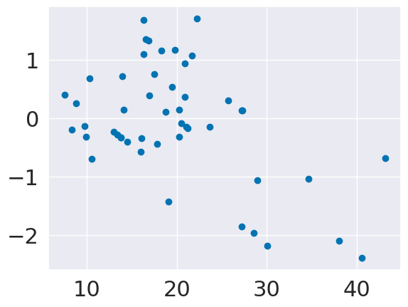
If our model was predicting uniformly well, these would be evenly distributed left to right.

16.3. Mutlivariate Regression

Recall the equation for a line:

\[ \hat{y} = mx+b\]

When we have multiple variables instead of a scalar \(x\) we can have a vector \(\mathbf{x}\) and instead of a single slope, we have a vector of coefficients \(\beta\)

\[ \hat{y} = \beta^T\mathbf{x} + \beta_0 \]

where \(\beta\) is the regr_db.coef_ and \(\beta_0\) is regr_db.intercept_ and that’s a vector multiplication and \(\hat{y}\) is y_pred and \(y\) is y_test.

In scalar form, a vector multiplication can be written like

\[ \hat{y} = \sum_{k=0}^d(x_k*\beta_k) + \beta_0\]

where there are \(d\) features, that is \(d\)= len(X_test[k]) and \(k\) indexed into it.

We are going to use 2 variables so it would be like:

\[ \hat{y} = \beta_1*x_1 + \beta_2*x_2 + \beta_0\]

tips_X = tips_df[['total_bill','size']]
tips_y = tips_df['tip']
tips_X_train, tips_X_test, tips_y_train,tips_y_test = train_test_split(tips_X,tips_y, random_state=5,train_size=.8)

We do not need the newaxis once we have more than one feature

tips_df[['total_bill','size']].values.shape

(244, 2)

tips_df[['total_bill','size']].values[:,np.newaxis].shape

(244, 1, 2)

regr_2feat = linear_model.LinearRegression()
regr_2feat.fit(tips_X_train,tips_y_train)

LinearRegression()

In a Jupyter environment, please rerun this cell to show the HTML representation or trust the notebook.
On GitHub, the HTML representation is unable to render, please try loading this page with nbviewer.org.

tips_y_pred_2 = regr_2feat.predict(tips_X_test)

regr_2feat.score(tips_X_test,tips_y_test)

-0.017340127412395878

tips_y_pred_2.shape, tips_y_test.shape,tips_X_test.shape

((49,), (49,), (49, 2))

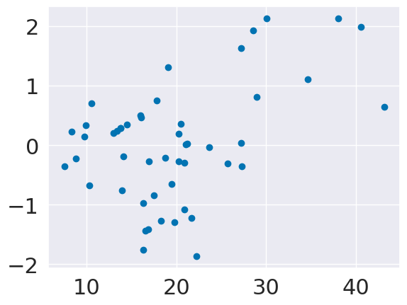
plt.scatter(tips_X_test['total_bill'],tips_y_pred_2-tips_y_test)

<matplotlib.collections.PathCollection at 0x7f8731b16cd0>

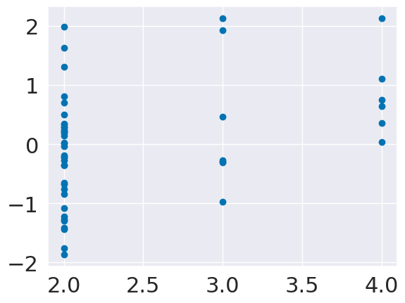
plt.scatter(tips_X_test['size'],tips_y_pred_2-tips_y_test)

<matplotlib.collections.PathCollection at 0x7f8731a8a3d0>

regr.coef_

array([0.11469301])

regr.intercept_

0.7426466344875204

tips_X_test.head()

	total_bill	size
55	19.49	2
191	19.81	2
210	30.06	3
96	27.28	2
163	13.81	2

np.sum(tips_X_test.values[0]*regr.coef_) +regr.intercept_

3.2073993683400492

tips_X_test.values[0][0]*regr.coef_[0] + tips_X_test.values[0][1]*regr.coef_[1] +regr.intercept_

---------------------------------------------------------------------------
IndexError                                Traceback (most recent call last)
Cell In[23], line 1
----> 1 tips_X_test.values[0][0]*regr.coef_[0] + tips_X_test.values[0][1]*regr.coef_[1] +regr.intercept_

IndexError: index 1 is out of bounds for axis 0 with size 1

tips_y_pred_2[0]

2.85825279437057

from sklearn.preprocessing import PolynomialFeatures

poly = PolynomialFeatures()

tips_X2_train = poly.fit_transform(tips_X_train)

regr2 = linear_model.LinearRegression()
regr2.fit(tips_X2_train,tips_y_train)

LinearRegression()

In a Jupyter environment, please rerun this cell to show the HTML representation or trust the notebook.
On GitHub, the HTML representation is unable to render, please try loading this page with nbviewer.org.

tips_X2_test = poly.fit_transform(tips_X_test)
tips_y_pred_sq = regr2.predict(tips_X2_test)

regr2.score(tips_X2_test,tips_y_test)

-0.041787136585906826

16.4. Questions After Class

Note

most were something like re-explain what just happened, so I did not answer them separately below, but made sure to add in detail above

16.4.1. where can I find good datasets for practice?

The UCI repository is the best place to start. Use the filters to select for regression, of moderate size, with numerical features.

You could also use a dataset with both numerical and categorical features and only us the numerical ones. Remember how in A2, I had you subset data to select for numerical features? There was a goal to that.

16.4.2. Does making the data quadratic help to find quadratic patterns, or does it simply give the model more data?

It finds quadratic patterns. That model has the same number of samples and, in a sense, the same amount of “data” but it has sort of a different view on the same data. Computing functions of our data is not considered to be generating more data, it’s thought of as a change of representation only.

When we added a second variable to the model, that was giving it more information about each sample and actually increasing the size of the data.

16.4.3. How specifically does the poly.fit_transform work?

For the details of the code, you can see the documentation. From there you can see the source for the PolynomialFeatures class. That inherits from the TransformerMixin which defines the fit_transform method which calls, in sequence the fit and transform methods as they are defined in the Polynomial features class. In this case the fit calculates the number of total output features and transform transforms the input features and outputs the new features.

Mathematically, we provide it a matrix, \(X\in \mathcal{R}^{n\times d}\) where the columns are vectors \(\mathbf{x_i}\in \mathcal{R}^{n}\) for \(i\in [0,\ldots,d]\) which means that there are \(d\) columns representing the original features and \(n\) samples. We get back a new matrix with columns: \([1, x_0, x_0^2, x_0*x_1,x_0*x_2, \ldots,x_0*x_d, x_1^2, x_1*x_2, \ldots, x_1*x_d,\ldots x_d^2]\)

This means that we can use the same algorithm to find the weights as we do for linear regression, using the transformed features.

A linear regression solver can sovle for the coefficients no matter what they are multiplied by.

16.4.4. Can you further explain the Y = B1x1 + B2x1^2 + B0 for both single variables and multiple variables?

16.4.5. I think I would just like another run down of the equation or maybe even just written in explanations