14. Predictions with niave Bayes and Decision Trees

import pandas as pd
import seaborn as sns
import numpy as np
import matplotlib.pylab as plt
from sklearn.model_selection import train_test_split
from sklearn.naive_bayes import GaussianNB
from sklearn import metrics
iris_df = sns.load_dataset('iris')

14.1. Classifying Irises

iris_df.head()

	sepal_length	sepal_width	petal_length	petal_width	species
0	5.1	3.5	1.4	0.2	setosa
1	4.9	3.0	1.4	0.2	setosa
2	4.7	3.2	1.3	0.2	setosa
3	4.6	3.1	1.5	0.2	setosa
4	5.0	3.6	1.4	0.2	setosa

Our goal is to predict the species from the measurements. In machine learning, we call the species the target variable. The three species of irises, setosa, virginica and versicolor are called the classes. Since the target variable is categorical, this prediction task is a classification problem.

Hint

I set the size of the training data here to 80% instead of the default 75%. I did not do this in class, but since the assignment asks you to change the training size, I included it here.

# dataset vars:
# 'petal_width',  'sepal_length','species', 'sepal_width','petal_length',
feature_vars = ['petal_width',  'sepal_length', 'sepal_width','petal_length',]
target_var = 'species'
X_train, X_test, y_train, y_test = train_test_split(iris_df[feature_vars],iris_df[target_var],random_state=0,train_size=.8)

Using the random_state makes it so that we get the same “random” set each type we run the code. see docs

Notice that in the training data the indices are randomly ordered unlike in the original DataFrame.

X_train.head()

	petal_width	sepal_length	sepal_width	petal_length
137	1.8	6.4	3.1	5.5
84	1.5	5.4	3.0	4.5
27	0.2	5.2	3.5	1.5
127	1.8	6.1	3.0	4.9
132	2.2	6.4	2.8	5.6

Next we can instantiate our estimator object which in this case is the GaussianNB

Note

The sklearn docs (and the docstring) include the reference to the exact implementation that they use, including the original research paper that discovered and evaluated that algorithm

gnb = GaussianNB()
gnb.fit(X_train,y_train)

GaussianNB()

In a Jupyter environment, please rerun this cell to show the HTML representation or trust the notebook.
On GitHub, the HTML representation is unable to render, please try loading this page with nbviewer.org.

We use the fit method to “learn” or find the values of the parameters.

gnb.score(X_test,y_test)

0.9666666666666667

Then we can check how well it works

y_pred = gnb.predict(X_test)

And see the atual predictions

y_pred == y_test

114     True
62      True
33      True
107     True
7       True
100     True
40      True
86      True
76      True
71      True
134    False
51      True
73      True
54      True
63      True
37      True
78      True
90      True
45      True
16      True
121     True
66      True
24      True
8       True
126     True
22      True
44      True
97      True
93      True
26      True
Name: species, dtype: bool

14.2. How does GNB make predictions?

we fit the Gaussian Naive Bayes, it computes a mean \(\theta\) and variance \(\sigma\) and adds them to model parameters in attributes

gnb.__dict__

{'priors': None,
 'var_smoothing': 1e-09,
 'classes_': array(['setosa', 'versicolor', 'virginica'], dtype='<U10'),
 'feature_names_in_': array(['petal_width', 'sepal_length', 'sepal_width', 'petal_length'],
       dtype=object),
 'n_features_in_': 4,
 'epsilon_': 3.159332638888889e-09,
 'theta_': array([[0.24102564, 5.02051282, 3.4025641 , 1.46153846],
        [1.32432432, 5.88648649, 2.76216216, 4.21621622],
        [2.03181818, 6.63863636, 2.98863636, 5.56590909]]),
 'var_': array([[0.01113741, 0.12932282, 0.1417883 , 0.02031559],
        [0.04075968, 0.26387144, 0.10397371, 0.23000731],
        [0.06444215, 0.38918905, 0.10782542, 0.29451963]]),
 'class_count_': array([39., 37., 44.]),
 'class_prior_': array([0.325     , 0.30833333, 0.36666667])}

The attributes of the estimator object (gbn) describe the data (eg the class list) and the model’s parameters. The theta_ (\(\theta\)) represents the mean and the var_ (\(\sigma\)) represents the variance of the distributions.

gnb.theta_

array([[0.24102564, 5.02051282, 3.4025641 , 1.46153846],
       [1.32432432, 5.88648649, 2.76216216, 4.21621622],
       [2.03181818, 6.63863636, 2.98863636, 5.56590909]])

Try it Yourself

Could you use what we learned about EDA to find the mean and variance of each feature for each species of flower?

Because the GaussianNB classifier calculates parameters that describe the assumed distribuiton of the data is is called a generative classifier. From a generative classifer, we can generate synthetic data that is from the distribution the classifer learned. If this data looks like our real data, then the model assumptions fit well.

Warning

the details of this math are not required understanding, but this describes the following block of code

Hint

to try understanding this block of code, try extracting pieces of it and running each piece individually. I built it up piece by piece adn then wrapped them all together.

To do this, we extract the mean and variance parameters from the model (gnb.theta_,gnb.sigma_) and zip them together to create an iterable object that in each iteration returns one value from each list (for th, sig in zip(gnb.theta_,gnb.sigma_)). We do this inside of a list comprehension and for each th,sig where th is from gnb.theta_ and sig is from gnb.sigma_ we use np.random.multivariate_normal to get 20 samples. In a general multivariate normal distribution the second parameter is actually a covariance matrix. This describes both the variance of each individual feature and the correlation of the features. Since Naive Bayes is Naive it assumes the features are independent or have 0 correlation. So, to create the matrix from the vector of variances we multiply by np.eye(4) which is the identity matrix or a matrix with 1 on the diagonal and 0 elsewhere. Finally we stack the groups for each species together with np.concatenate (like pd.concat but works on numpy objects and np.random.multivariate_normal returns numpy arrays not data frames) and put all of that in a DataFrame using the feature names as the columns.

Then we add a species column, by repeating each species 20 times [c]*N for c in gnb.classes_ and then unpack that into a single list instead of as list of lists.

N = 50
gnb_df = pd.DataFrame(np.concatenate([np.random.multivariate_normal(th, sig*np.eye(4),N)
                 for th, sig in zip(gnb.theta_,gnb.var_)]),
                 columns = gnb.feature_names_in_)
gnb_df['species'] = [ci for cl in [[c]*N for c in gnb.classes_] for ci in cl]
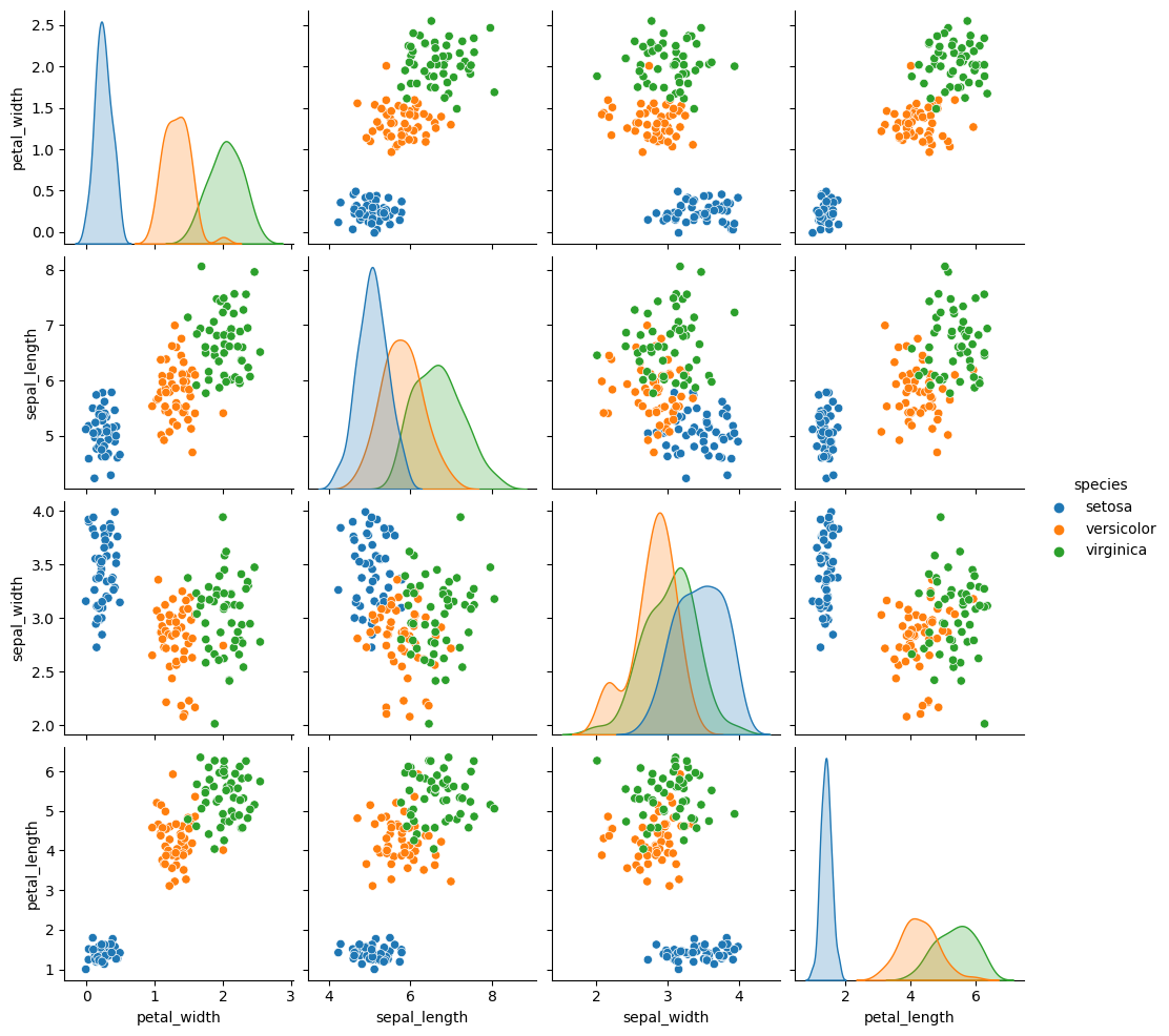
sns.pairplot(data =gnb_df, hue='species')

<seaborn.axisgrid.PairGrid at 0x7f5d1087c4f0>

Further Reading

There are other classifiers that use roughly the same model but don’t make the naive assumption. The more flexible is called Quadratic Discriminant Analysis.

• mathematical formulation for both

• QDA code

• LDA code

sns.pairplot(data=iris_df,hue='species')

<seaborn.axisgrid.PairGrid at 0x7f5cd106f130>

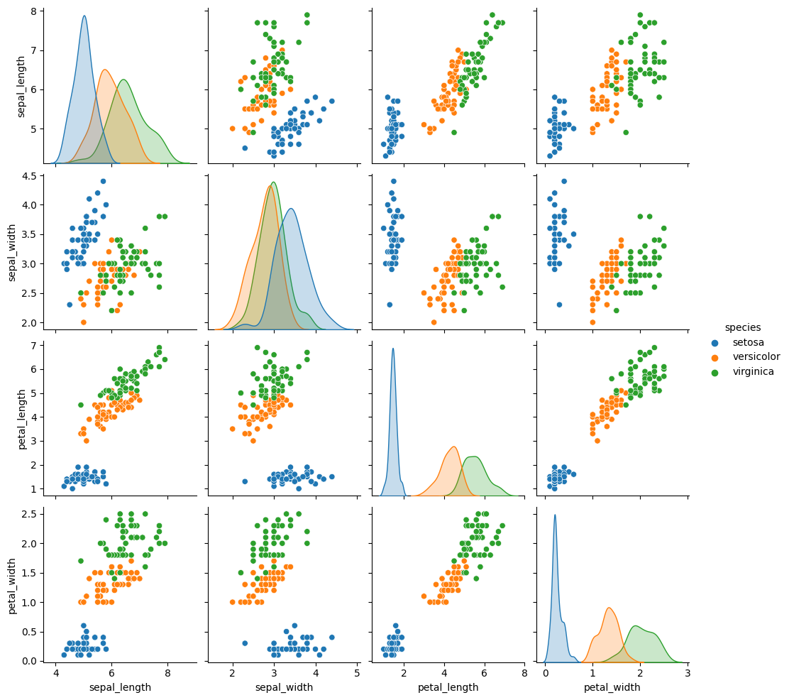
This one looks pretty close to the actual data. The biggest difference is that these data are all in uniformly circular-ish blobs and the ones above are not.
That means that the naive assumption doesn’t hold perfectly on this data.

When we use the predict method, it uses those parameters to calculate the likelihood of the sample according to a Gaussian distribution (normal) for each class and then calculates the probability of the sample belonging to each class and returns the one with the highest probability.

14.3. Interpretting probabilities

We can look directly at the probabilities

gnb.predict_proba(X_test)

array([[1.63380783e-232, 2.18878438e-006, 9.99997811e-001],
       [1.82640391e-082, 9.99998304e-001, 1.69618390e-006],
       [1.00000000e+000, 7.10250510e-019, 3.65449801e-028],
       [1.58508262e-305, 1.04649020e-006, 9.99998954e-001],
       [1.00000000e+000, 8.59168655e-017, 4.22159374e-027],
       [6.39815011e-321, 1.56450314e-010, 1.00000000e+000],
       [1.00000000e+000, 1.09797313e-016, 5.30276557e-027],
       [1.25122812e-146, 7.74052109e-001, 2.25947891e-001],
       [5.34357526e-150, 9.07564955e-001, 9.24350453e-002],
       [5.67261712e-093, 9.99882109e-001, 1.17891111e-004],
       [2.38651144e-210, 5.29609631e-001, 4.70390369e-001],
       [8.12047631e-132, 9.43762575e-001, 5.62374248e-002],
       [5.25177109e-132, 9.98864361e-001, 1.13563851e-003],
       [1.24498038e-139, 9.49838641e-001, 5.01613586e-002],
       [4.08232760e-140, 9.88043864e-001, 1.19561365e-002],
       [1.00000000e+000, 7.12837229e-019, 4.10162749e-029],
       [4.19553996e-131, 9.87944980e-001, 1.20550201e-002],
       [4.13286716e-111, 9.99942383e-001, 5.76167389e-005],
       [1.00000000e+000, 2.24933112e-015, 3.63624519e-026],
       [1.00000000e+000, 9.86750131e-016, 2.42355087e-025],
       [1.85930865e-186, 1.66966805e-002, 9.83303319e-001],
       [8.83060167e-130, 9.92757232e-001, 7.24276827e-003],
       [1.00000000e+000, 4.26380344e-013, 4.34222344e-023],
       [1.00000000e+000, 1.28045851e-016, 1.26708019e-027],
       [2.43739221e-168, 1.83516225e-001, 8.16483775e-001],
       [1.00000000e+000, 2.62431469e-018, 6.72573168e-029],
       [1.00000000e+000, 3.20605389e-011, 1.52433420e-020],
       [2.20964201e-110, 9.99291229e-001, 7.08771072e-004],
       [1.39297338e-046, 9.99999972e-001, 2.81392389e-008],
       [1.00000000e+000, 1.85943966e-013, 1.58833385e-023]])

We can see that for most of these one value is close to one and the others are close to zero. One way to emphasize this is to round them.

y_prob = gnb.predict_proba(X_test)
np.round(y_prob,2)

array([[0.  , 0.  , 1.  ],
       [0.  , 1.  , 0.  ],
       [1.  , 0.  , 0.  ],
       [0.  , 0.  , 1.  ],
       [1.  , 0.  , 0.  ],
       [0.  , 0.  , 1.  ],
       [1.  , 0.  , 0.  ],
       [0.  , 0.77, 0.23],
       [0.  , 0.91, 0.09],
       [0.  , 1.  , 0.  ],
       [0.  , 0.53, 0.47],
       [0.  , 0.94, 0.06],
       [0.  , 1.  , 0.  ],
       [0.  , 0.95, 0.05],
       [0.  , 0.99, 0.01],
       [1.  , 0.  , 0.  ],
       [0.  , 0.99, 0.01],
       [0.  , 1.  , 0.  ],
       [1.  , 0.  , 0.  ],
       [1.  , 0.  , 0.  ],
       [0.  , 0.02, 0.98],
       [0.  , 0.99, 0.01],
       [1.  , 0.  , 0.  ],
       [1.  , 0.  , 0.  ],
       [0.  , 0.18, 0.82],
       [1.  , 0.  , 0.  ],
       [1.  , 0.  , 0.  ],
       [0.  , 1.  , 0.  ],
       [0.  , 1.  , 0.  ],
       [1.  , 0.  , 0.  ]])

Important

The following did not happen in class, but I added more explanation so tha it is more clear.

These are hard to interpret as is, one option is to plot them

# make the prbabilities into a dataframe labeled with classes & make the index a separate column
prob_df = pd.DataFrame(data = gnb.predict_proba(X_test), columns = gnb.classes_ ).reset_index()
# add the predictions
prob_df['predicted_species'] = y_pred
prob_df['true_species'] = y_test.values
# for plotting, make a column that combines the index & prediction
pred_text = lambda r: str( r['index']) + ',' + r['predicted_species']
prob_df['i,pred'] = prob_df.apply(pred_text,axis=1)
# same for ground truth
true_text = lambda r: str( r['index']) + ',' + r['true_species']
prob_df['correct'] = prob_df['predicted_species'] == prob_df['true_species']
# a dd a column for which are correct
prob_df['i,true'] = prob_df.apply(true_text,axis=1)
prob_df_melted = prob_df.melt(id_vars =[ 'index', 'predicted_species','true_species','i,pred','i,true','correct'],value_vars = gnb.classes_,
                             var_name = target_var, value_name = 'probability')
prob_df_melted.head()

	index	predicted_species	true_species	i,pred	i,true	correct	species	probability
0	0	virginica	virginica	0,virginica	0,virginica	True	setosa	1.633808e-232
1	1	versicolor	versicolor	1,versicolor	1,versicolor	True	setosa	1.826404e-82
2	2	setosa	setosa	2,setosa	2,setosa	True	setosa	1.000000e+00
3	3	virginica	virginica	3,virginica	3,virginica	True	setosa	1.585083e-305
4	4	setosa	setosa	4,setosa	4,setosa	True	setosa	1.000000e+00

Now we have a data frame where each rown is one the probability of one sample belonging to one class. So there’s a total of number_of_samples*number_of_classes rows

prob_df_melted.shape

(90, 8)

len(y_pred)*len(gnb.classes_)

90

One way to look at these is to, for each sample in the test set, make a bar chart of the probability it belongs to each class. We added to the data frame information so that we can plot this with the true class in the title using col = 'i,true'

Tip

I used set_theme to change both the fond size and the color palette. Seaborn has a detailed guide for choosing colors. The colorblind palette uses colors that are distinguishable under most common forms of color blindness.

sns.set_theme(font_scale=2, palette= "colorblind")
# plot a bar graph for each point labeled with the prediction
sns.catplot(data =prob_df_melted, x = 'species', y='probability' ,col ='i,true',
            col_wrap=5,kind='bar')

<seaborn.axisgrid.FacetGrid at 0x7f5ccd604790>

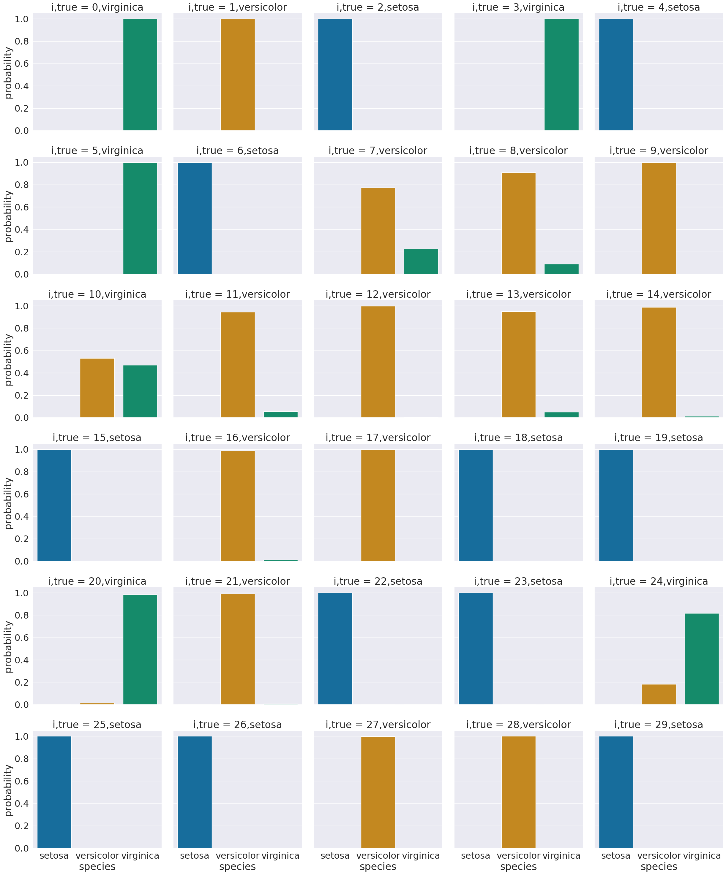
We see that most sampples have nearly all of their probability mass (all probabiilties in a distribution sum (or integrate if continuous) to 1, but a few samples are not.

14.4. What about a harder dataset?

Using a toy dataset here shows an easy to see challenge for the classifier that we have seen so far. Real datasets will be hard in different ways, and since they’re higher dimensional, it’s harder to visualize the cause.

corner_data = 'https://raw.githubusercontent.com/rhodyprog4ds/06-naive-bayes/f425ba121cc0c4dd8bcaa7ebb2ff0b40b0b03bff/data/dataset6.csv'
df6= pd.read_csv(corner_data,usecols=[1,2,3])
gnb_corners = GaussianNB()
sns.pairplot(data=df6, hue='char',hue_order=['A','B'])

<seaborn.axisgrid.PairGrid at 0x7f5ccd7a4250>

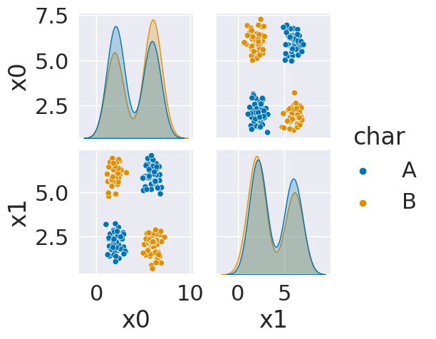
As we can see in this dataset, these classes are quite separated. We might expect a pretty good performance.

df6.head()

	x0	x1	char
0	6.14	2.10	B
1	2.22	2.39	A
2	2.27	5.44	B
3	1.03	3.19	A
4	2.25	1.71	A

Xcorners_train, Xcorners_test, ycorners_train, ycorners_test = train_test_split(
                df6.drop(columns='char'),df6['char'])
gnb_corners.fit(Xcorners_train,ycorners_train)

GaussianNB()

In a Jupyter environment, please rerun this cell to show the HTML representation or trust the notebook.
On GitHub, the HTML representation is unable to render, please try loading this page with nbviewer.org.

gnb_corners.score(Xcorners_test,ycorners_test)

0.66

But we do not get a very good classification score.

To see why, we can look at what it learned.

N = 100
gnb_corners_df = pd.DataFrame(np.concatenate([np.random.multivariate_normal(th, sig*np.eye(2),N)
         for th, sig in zip(gnb_corners.theta_,gnb.sigma_)]),
         columns = ['x0','x1'])
gnb_corners_df['char'] = [ci for cl in [[c]*N for c in gnb_corners.classes_] for ci in cl]

sns.pairplot(data =gnb_corners_df, hue='char',hue_order=['A','B'])

---------------------------------------------------------------------------
AttributeError                            Traceback (most recent call last)
Cell In[23], line 3
      1 N = 100
      2 gnb_corners_df = pd.DataFrame(np.concatenate([np.random.multivariate_normal(th, sig*np.eye(2),N)
----> 3          for th, sig in zip(gnb_corners.theta_,gnb.sigma_)]),
      4          columns = ['x0','x1'])
      5 gnb_corners_df['char'] = [ci for cl in [[c]*N for c in gnb_corners.classes_] for ci in cl]
      7 sns.pairplot(data =gnb_corners_df, hue='char',hue_order=['A','B'])

AttributeError: 'GaussianNB' object has no attribute 'sigma_'

14.5. Decision Trees

The Gaussian Naive Bayes model we have seen so far, worked on this really well separated Gaussian distributed data. Not all data is that easy to classify. Sometimes coming up with a description of the data for a generative model is hard and it might not even be important. A scientist will find that valuable, but it is not always needed. Another way to think about classification is to focus on writing a rule (or set of rules) for determining the label from the features. This type of classifier is called discriminative, because it focuses on discriminating (in the literal, differentiate sense, not the socially loaded differentiate on the basis of an attribute of the person in unfair ways sense) between the classes.

This data does not fit the assumptions of the Niave Bayes model, but a decision tree has a different rule. It can be more complex, but for the scikit learn one relies on splitting the data at a series of points along one axis at a time.

It is a discriminative model, because it describes how to discriminate (in the sense of differentiate) between the classes.

from sklearn import tree

The sklearn estimator objects (that correspond to different models) all have the same API, so the fit, predict, and score methods are the same as above. We will see this also in regression and clustering. What each method does in terms of the specific calculations will vary depending on the model, but they’re always there.

dt = tree.DecisionTreeClassifier()
dt.fit(Xcorners_train,ycorners_train)

DecisionTreeClassifier()

In a Jupyter environment, please rerun this cell to show the HTML representation or trust the notebook.
On GitHub, the HTML representation is unable to render, please try loading this page with nbviewer.org.

dt.score(Xcorners_test,ycorners_test)

1.0

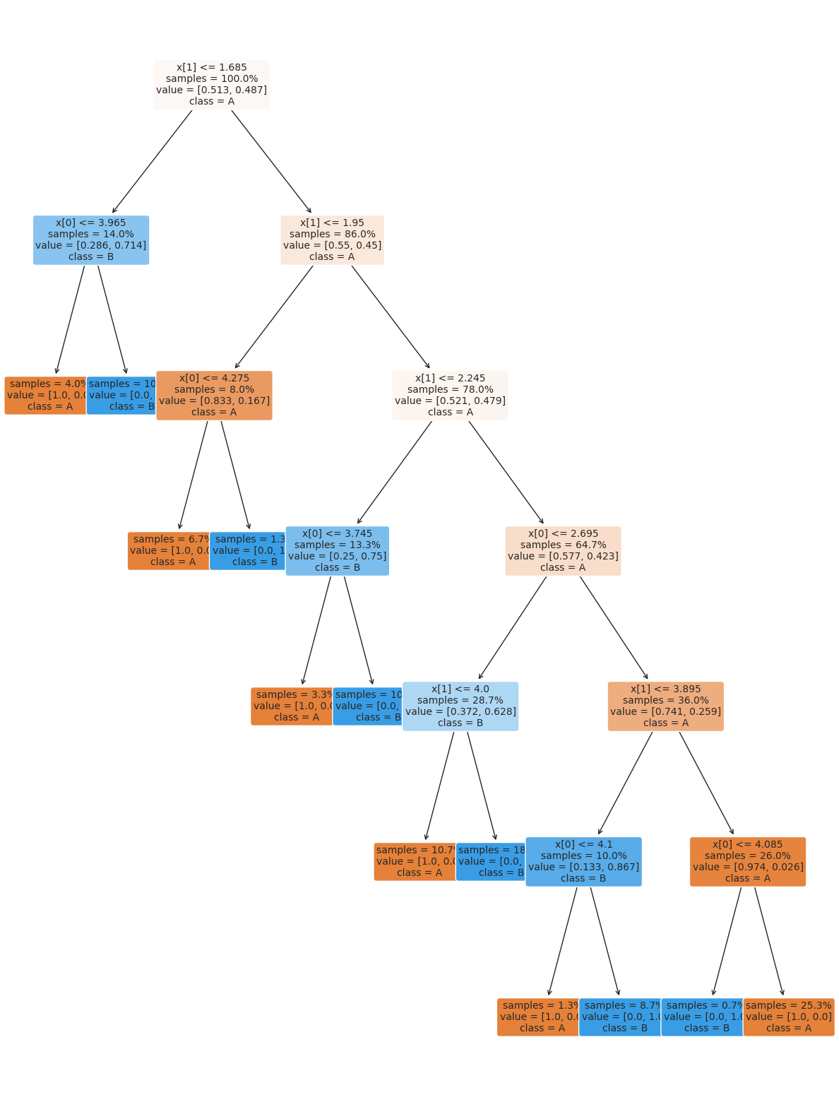
The tree module also allows you to plot the tree to examine it.

plt.figure(figsize=(15,20))
tree.plot_tree(dt, rounded =True, class_names = ['A','B'],
            proportion=True, filled =True, impurity=False,fontsize=10)

[Text(0.246875, 0.9285714285714286, 'x[1] <= 1.685\nsamples = 100.0%\nvalue = [0.513, 0.487]\nclass = A'),
 Text(0.1, 0.7857142857142857, 'x[0] <= 3.965\nsamples = 14.0%\nvalue = [0.286, 0.714]\nclass = B'),
 Text(0.05, 0.6428571428571429, 'samples = 4.0%\nvalue = [1.0, 0.0]\nclass = A'),
 Text(0.15, 0.6428571428571429, 'samples = 10.0%\nvalue = [0.0, 1.0]\nclass = B'),
 Text(0.39375, 0.7857142857142857, 'x[1] <= 1.95\nsamples = 86.0%\nvalue = [0.55, 0.45]\nclass = A'),
 Text(0.25, 0.6428571428571429, 'x[0] <= 4.275\nsamples = 8.0%\nvalue = [0.833, 0.167]\nclass = A'),
 Text(0.2, 0.5, 'samples = 6.7%\nvalue = [1.0, 0.0]\nclass = A'),
 Text(0.3, 0.5, 'samples = 1.3%\nvalue = [0.0, 1.0]\nclass = B'),
 Text(0.5375, 0.6428571428571429, 'x[1] <= 2.245\nsamples = 78.0%\nvalue = [0.521, 0.479]\nclass = A'),
 Text(0.4, 0.5, 'x[0] <= 3.745\nsamples = 13.3%\nvalue = [0.25, 0.75]\nclass = B'),
 Text(0.35, 0.35714285714285715, 'samples = 3.3%\nvalue = [1.0, 0.0]\nclass = A'),
 Text(0.45, 0.35714285714285715, 'samples = 10.0%\nvalue = [0.0, 1.0]\nclass = B'),
 Text(0.675, 0.5, 'x[0] <= 2.695\nsamples = 64.7%\nvalue = [0.577, 0.423]\nclass = A'),
 Text(0.55, 0.35714285714285715, 'x[1] <= 4.0\nsamples = 28.7%\nvalue = [0.372, 0.628]\nclass = B'),
 Text(0.5, 0.21428571428571427, 'samples = 10.7%\nvalue = [1.0, 0.0]\nclass = A'),
 Text(0.6, 0.21428571428571427, 'samples = 18.0%\nvalue = [0.0, 1.0]\nclass = B'),
 Text(0.8, 0.35714285714285715, 'x[1] <= 3.895\nsamples = 36.0%\nvalue = [0.741, 0.259]\nclass = A'),
 Text(0.7, 0.21428571428571427, 'x[0] <= 4.1\nsamples = 10.0%\nvalue = [0.133, 0.867]\nclass = B'),
 Text(0.65, 0.07142857142857142, 'samples = 1.3%\nvalue = [1.0, 0.0]\nclass = A'),
 Text(0.75, 0.07142857142857142, 'samples = 8.7%\nvalue = [0.0, 1.0]\nclass = B'),
 Text(0.9, 0.21428571428571427, 'x[0] <= 4.085\nsamples = 26.0%\nvalue = [0.974, 0.026]\nclass = A'),
 Text(0.85, 0.07142857142857142, 'samples = 0.7%\nvalue = [0.0, 1.0]\nclass = B'),
 Text(0.95, 0.07142857142857142, 'samples = 25.3%\nvalue = [1.0, 0.0]\nclass = A')]

Note

On the iris dataset, the sklearn docs include a diagram showing the decision boundary You should be able to modify this for another classifier.

14.6. Setting Classifier Parameters

The decision tree we had above has a lot more layers than we would expect. This is really simple data so we still got perfect classification. However, the more complex the model, the more risk that it will learn something noisy about the training data that doesn’t hold up in the test set.

Fortunately, we can control the parameters to make it find a simpler decision boundary.

dt2 = tree.DecisionTreeClassifier(max_depth=2)
dt2.fit(Xcorners_train,ycorners_train)
dt2.score(Xcorners_test,ycorners_test)

0.56

We might need to play with different parameters to get it just how we want it. A simpler model can be better because it is easier to understand and sometimes will generalize, or apply to new data, better.

14.7. Example Loading UCI data

Hint

This is a hint for a7

Remember in classification, we predict a cateogrical variable from related continuous feature variables.

The data is a .data file, but if you look at it, it will actually be comma, tab, or space delimited, so read_csv will work.

pd.read_csv('glass.data').head()

---------------------------------------------------------------------------
FileNotFoundError                         Traceback (most recent call last)
Cell In[29], line 1
----> 1 pd.read_csv('glass.data').head()

File /opt/hostedtoolcache/Python/3.8.16/x64/lib/python3.8/site-packages/pandas/io/parsers/readers.py:912, in read_csv(filepath_or_buffer, sep, delimiter, header, names, index_col, usecols, dtype, engine, converters, true_values, false_values, skipinitialspace, skiprows, skipfooter, nrows, na_values, keep_default_na, na_filter, verbose, skip_blank_lines, parse_dates, infer_datetime_format, keep_date_col, date_parser, date_format, dayfirst, cache_dates, iterator, chunksize, compression, thousands, decimal, lineterminator, quotechar, quoting, doublequote, escapechar, comment, encoding, encoding_errors, dialect, on_bad_lines, delim_whitespace, low_memory, memory_map, float_precision, storage_options, dtype_backend)
    899 kwds_defaults = _refine_defaults_read(
    900     dialect,
    901     delimiter,
   (...)
    908     dtype_backend=dtype_backend,
    909 )
    910 kwds.update(kwds_defaults)
--> 912 return _read(filepath_or_buffer, kwds)

File /opt/hostedtoolcache/Python/3.8.16/x64/lib/python3.8/site-packages/pandas/io/parsers/readers.py:577, in _read(filepath_or_buffer, kwds)
    574 _validate_names(kwds.get("names", None))
    576 # Create the parser.
--> 577 parser = TextFileReader(filepath_or_buffer, **kwds)
    579 if chunksize or iterator:
    580     return parser

File /opt/hostedtoolcache/Python/3.8.16/x64/lib/python3.8/site-packages/pandas/io/parsers/readers.py:1407, in TextFileReader.__init__(self, f, engine, **kwds)
   1404     self.options["has_index_names"] = kwds["has_index_names"]
   1406 self.handles: IOHandles | None = None
-> 1407 self._engine = self._make_engine(f, self.engine)

File /opt/hostedtoolcache/Python/3.8.16/x64/lib/python3.8/site-packages/pandas/io/parsers/readers.py:1661, in TextFileReader._make_engine(self, f, engine)
   1659     if "b" not in mode:
   1660         mode += "b"
-> 1661 self.handles = get_handle(
   1662     f,
   1663     mode,
   1664     encoding=self.options.get("encoding", None),
   1665     compression=self.options.get("compression", None),
   1666     memory_map=self.options.get("memory_map", False),
   1667     is_text=is_text,
   1668     errors=self.options.get("encoding_errors", "strict"),
   1669     storage_options=self.options.get("storage_options", None),
   1670 )
   1671 assert self.handles is not None
   1672 f = self.handles.handle

File /opt/hostedtoolcache/Python/3.8.16/x64/lib/python3.8/site-packages/pandas/io/common.py:859, in get_handle(path_or_buf, mode, encoding, compression, memory_map, is_text, errors, storage_options)
    854 elif isinstance(handle, str):
    855     # Check whether the filename is to be opened in binary mode.
    856     # Binary mode does not support 'encoding' and 'newline'.
    857     if ioargs.encoding and "b" not in ioargs.mode:
    858         # Encoding
--> 859         handle = open(
    860             handle,
    861             ioargs.mode,
    862             encoding=ioargs.encoding,
    863             errors=errors,
    864             newline="",
    865         )
    866     else:
    867         # Binary mode
    868         handle = open(handle, ioargs.mode)

FileNotFoundError: [Errno 2] No such file or directory: 'glass.data'

I would notice that the first row is data, not headers so I would go to the glass.names file to find the column names

in the glass.names file there is a lot of other information, but the important part is a list of the columns:

   1. Id number: 1 to 214
   2. RI: refractive index
   3. Na: Sodium (unit measurement: weight percent in corresponding oxide, as 
                  are attributes 4-10)
   4. Mg: Magnesium
   5. Al: Aluminum
   6. Si: Silicon
   7. K: Potassium
   8. Ca: Calcium
   9. Ba: Barium
  10. Fe: Iron
  11. Type of glass:

If I were going to work on this, I would copy that section into a string and then delete that () section after sodium.

names= '''   1. Id number: 1 to 214
   2. RI: refractive index
   3. Na: Sodium 
   4. Mg: Magnesium
   5. Al: Aluminum
   6. Si: Silicon
   7. K: Potassium
   8. Ca: Calcium
   9. Ba: Barium
  10. Fe: Iron
  11. Type of glass:'''

Then instead of cutting each one to make a list manually, I might do the following:

col_names = [cn.split('.')[1].split(':')[0].strip().replace(' ','_') 
             for cn in names.split('\n')]
col_names

['Id_number',
 'RI',
 'Na',
 'Mg',
 'Al',
 'Si',
 'K',
 'Ca',
 'Ba',
 'Fe',
 'Type_of_glass']

pd.read_csv('glass.data',names=col_names).head()

---------------------------------------------------------------------------
FileNotFoundError                         Traceback (most recent call last)
Cell In[32], line 1
----> 1 pd.read_csv('glass.data',names=col_names).head()

File /opt/hostedtoolcache/Python/3.8.16/x64/lib/python3.8/site-packages/pandas/io/parsers/readers.py:912, in read_csv(filepath_or_buffer, sep, delimiter, header, names, index_col, usecols, dtype, engine, converters, true_values, false_values, skipinitialspace, skiprows, skipfooter, nrows, na_values, keep_default_na, na_filter, verbose, skip_blank_lines, parse_dates, infer_datetime_format, keep_date_col, date_parser, date_format, dayfirst, cache_dates, iterator, chunksize, compression, thousands, decimal, lineterminator, quotechar, quoting, doublequote, escapechar, comment, encoding, encoding_errors, dialect, on_bad_lines, delim_whitespace, low_memory, memory_map, float_precision, storage_options, dtype_backend)
    899 kwds_defaults = _refine_defaults_read(
    900     dialect,
    901     delimiter,
   (...)
    908     dtype_backend=dtype_backend,
    909 )
    910 kwds.update(kwds_defaults)
--> 912 return _read(filepath_or_buffer, kwds)

File /opt/hostedtoolcache/Python/3.8.16/x64/lib/python3.8/site-packages/pandas/io/parsers/readers.py:577, in _read(filepath_or_buffer, kwds)
    574 _validate_names(kwds.get("names", None))
    576 # Create the parser.
--> 577 parser = TextFileReader(filepath_or_buffer, **kwds)
    579 if chunksize or iterator:
    580     return parser

File /opt/hostedtoolcache/Python/3.8.16/x64/lib/python3.8/site-packages/pandas/io/parsers/readers.py:1407, in TextFileReader.__init__(self, f, engine, **kwds)
   1404     self.options["has_index_names"] = kwds["has_index_names"]
   1406 self.handles: IOHandles | None = None
-> 1407 self._engine = self._make_engine(f, self.engine)

File /opt/hostedtoolcache/Python/3.8.16/x64/lib/python3.8/site-packages/pandas/io/parsers/readers.py:1661, in TextFileReader._make_engine(self, f, engine)
   1659     if "b" not in mode:
   1660         mode += "b"
-> 1661 self.handles = get_handle(
   1662     f,
   1663     mode,
   1664     encoding=self.options.get("encoding", None),
   1665     compression=self.options.get("compression", None),
   1666     memory_map=self.options.get("memory_map", False),
   1667     is_text=is_text,
   1668     errors=self.options.get("encoding_errors", "strict"),
   1669     storage_options=self.options.get("storage_options", None),
   1670 )
   1671 assert self.handles is not None
   1672 f = self.handles.handle

File /opt/hostedtoolcache/Python/3.8.16/x64/lib/python3.8/site-packages/pandas/io/common.py:859, in get_handle(path_or_buf, mode, encoding, compression, memory_map, is_text, errors, storage_options)
    854 elif isinstance(handle, str):
    855     # Check whether the filename is to be opened in binary mode.
    856     # Binary mode does not support 'encoding' and 'newline'.
    857     if ioargs.encoding and "b" not in ioargs.mode:
    858         # Encoding
--> 859         handle = open(
    860             handle,
    861             ioargs.mode,
    862             encoding=ioargs.encoding,
    863             errors=errors,
    864             newline="",
    865         )
    866     else:
    867         # Binary mode
    868         handle = open(handle, ioargs.mode)

FileNotFoundError: [Errno 2] No such file or directory: 'glass.data'

This looks good, so I would save it now. I might even save is as csv

glass_df = pd.read_csv('glass.data',names=col_names)

---------------------------------------------------------------------------
FileNotFoundError                         Traceback (most recent call last)
Cell In[33], line 1
----> 1 glass_df = pd.read_csv('glass.data',names=col_names)

File /opt/hostedtoolcache/Python/3.8.16/x64/lib/python3.8/site-packages/pandas/io/parsers/readers.py:912, in read_csv(filepath_or_buffer, sep, delimiter, header, names, index_col, usecols, dtype, engine, converters, true_values, false_values, skipinitialspace, skiprows, skipfooter, nrows, na_values, keep_default_na, na_filter, verbose, skip_blank_lines, parse_dates, infer_datetime_format, keep_date_col, date_parser, date_format, dayfirst, cache_dates, iterator, chunksize, compression, thousands, decimal, lineterminator, quotechar, quoting, doublequote, escapechar, comment, encoding, encoding_errors, dialect, on_bad_lines, delim_whitespace, low_memory, memory_map, float_precision, storage_options, dtype_backend)
    899 kwds_defaults = _refine_defaults_read(
    900     dialect,
    901     delimiter,
   (...)
    908     dtype_backend=dtype_backend,
    909 )
    910 kwds.update(kwds_defaults)
--> 912 return _read(filepath_or_buffer, kwds)

File /opt/hostedtoolcache/Python/3.8.16/x64/lib/python3.8/site-packages/pandas/io/parsers/readers.py:577, in _read(filepath_or_buffer, kwds)
    574 _validate_names(kwds.get("names", None))
    576 # Create the parser.
--> 577 parser = TextFileReader(filepath_or_buffer, **kwds)
    579 if chunksize or iterator:
    580     return parser

File /opt/hostedtoolcache/Python/3.8.16/x64/lib/python3.8/site-packages/pandas/io/parsers/readers.py:1407, in TextFileReader.__init__(self, f, engine, **kwds)
   1404     self.options["has_index_names"] = kwds["has_index_names"]
   1406 self.handles: IOHandles | None = None
-> 1407 self._engine = self._make_engine(f, self.engine)

File /opt/hostedtoolcache/Python/3.8.16/x64/lib/python3.8/site-packages/pandas/io/parsers/readers.py:1661, in TextFileReader._make_engine(self, f, engine)
   1659     if "b" not in mode:
   1660         mode += "b"
-> 1661 self.handles = get_handle(
   1662     f,
   1663     mode,
   1664     encoding=self.options.get("encoding", None),
   1665     compression=self.options.get("compression", None),
   1666     memory_map=self.options.get("memory_map", False),
   1667     is_text=is_text,
   1668     errors=self.options.get("encoding_errors", "strict"),
   1669     storage_options=self.options.get("storage_options", None),
   1670 )
   1671 assert self.handles is not None
   1672 f = self.handles.handle

File /opt/hostedtoolcache/Python/3.8.16/x64/lib/python3.8/site-packages/pandas/io/common.py:859, in get_handle(path_or_buf, mode, encoding, compression, memory_map, is_text, errors, storage_options)
    854 elif isinstance(handle, str):
    855     # Check whether the filename is to be opened in binary mode.
    856     # Binary mode does not support 'encoding' and 'newline'.
    857     if ioargs.encoding and "b" not in ioargs.mode:
    858         # Encoding
--> 859         handle = open(
    860             handle,
    861             ioargs.mode,
    862             encoding=ioargs.encoding,
    863             errors=errors,
    864             newline="",
    865         )
    866     else:
    867         # Binary mode
    868         handle = open(handle, ioargs.mode)

FileNotFoundError: [Errno 2] No such file or directory: 'glass.data'

glass_df['Type_of_glass'].value_counts()

---------------------------------------------------------------------------
NameError                                 Traceback (most recent call last)
Cell In[34], line 1
----> 1 glass_df['Type_of_glass'].value_counts()

NameError: name 'glass_df' is not defined

This shows that there are 6 classes, and they are different sizes.