17. Comparing Classification and Clustering Data#
Datasets for classification must have a target varialbe observed, but we can drop it to use it for clustering
17.1. KMeans review#
clustering goal: find groups of samples that are similar
k-means assumption: a fixed number (\(k\)) of means will describe the data enough to find the groups
17.2. Clustering with Sci-kit Learn#
import seaborn as sns
import numpy as np
from sklearn import datasets
from sklearn.cluster import KMeans
from sklearn import metrics
import pandas as pd
sns.set_theme(palette='colorblind')

# set global random seed so that the notes are the same each time the site builds
np.random.seed(1103)
%matplotlib inline
Load the iris data from seaborn
iris_df = sns.load_dataset('iris')
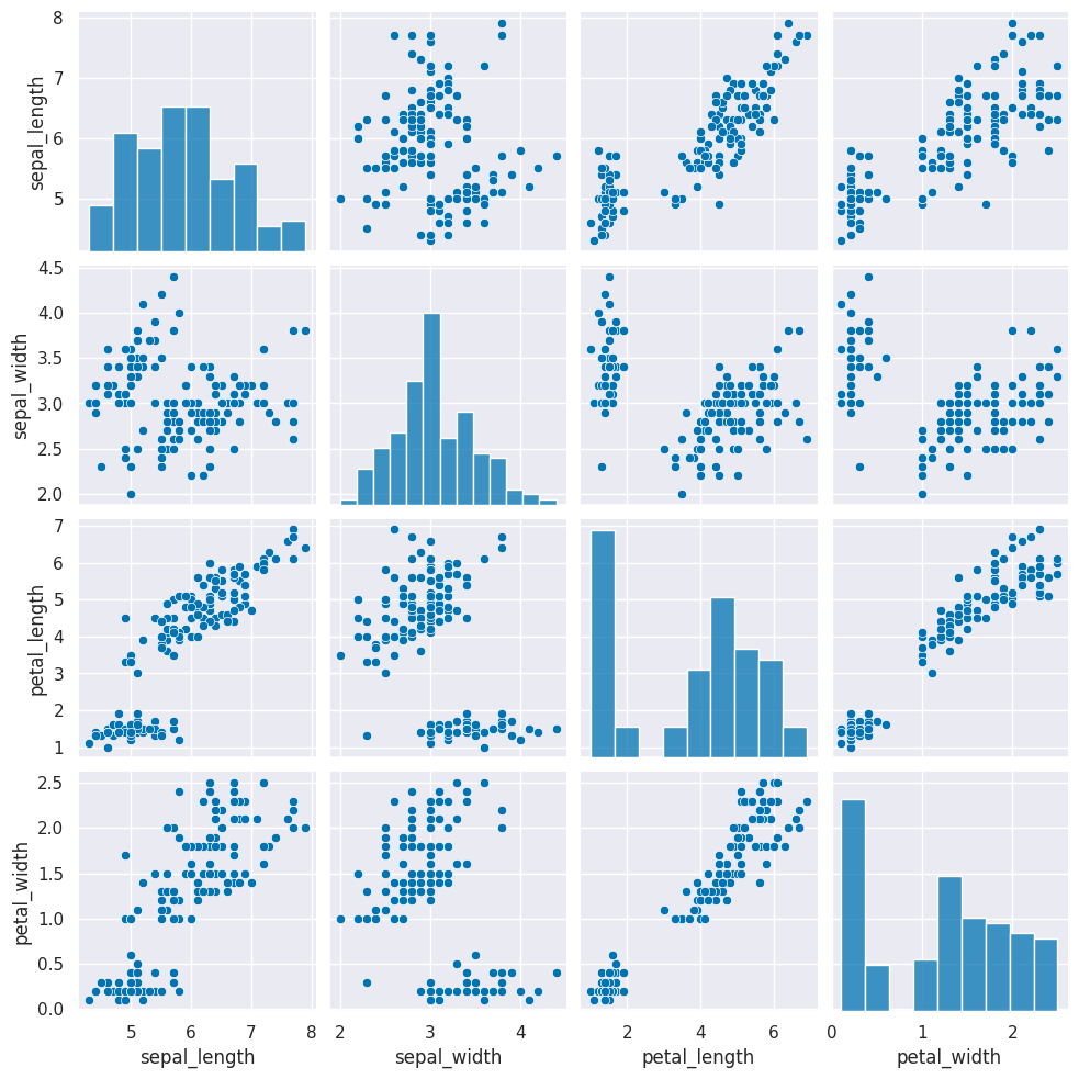
What plotting command will Create a grid of scatterplots of the data, without coloring the points differently
sns.pairplot(iris_df)
<seaborn.axisgrid.PairGrid at 0x7fb753312f10>
Next we need to create a copy of the data that’s appropriate for clustering. Remember that clustering is unsupervised so it doesn’t have a target variable. We also can do clustering on the data with or without splitting into test/train splits, since it doesn’t use a target variable, we can evaluate how good the clusters it finds are on the actual data that it learned from.
We can either pick the measurements out or drop the species column. remember most data frame operations return a copy of the dataframe.
We’ll do this by picking out the measurement columns, but we could also drop the species for now.
measurement_cols = ['sepal_length','petal_length','sepal_width','petal_width']
iris_X = iris_df[measurement_cols]
Alternate, equivalent
# iris_X =iris_df.drop(columns=['species']) # equivalent to above
Create a Kmeans estimator object with 3 clusters, since we know that the iris data has 3 species of flowers. We refer to these three groups as classes in classification (the goal is to label the classes…) and in clustering we sometimes borrow that word. Sometimes, clustering literature will be more abstract and refer to partitions, this is especially common in more mathematical/statistical work as opposed to algorithmic work on clustering.
km = KMeans(n_clusters=3)
We dropped the column that tells us which of the three classes that each sample(row) belongs to. We still have data from three species of flows.
Hint
use shift+tab or another jupyter help to figure out what the parameter names are for any function or class you’re working with.
Since we don’t have separate test and train data, we can use the fit_predict method. This is what the kmeans algorithm always does anyway, it both learns the means and the assignment (or prediction) for each sample at the same time.
Use the fit_predict method and look at what it outputs.
km.fit_predict(iris_X)
/opt/hostedtoolcache/Python/3.8.16/x64/lib/python3.8/site-packages/sklearn/cluster/_kmeans.py:870: FutureWarning: The default value of `n_init` will change from 10 to 'auto' in 1.4. Set the value of `n_init` explicitly to suppress the warning
  warnings.warn(
array([0, 0, 0, 0, 0, 0, 0, 0, 0, 0, 0, 0, 0, 0, 0, 0, 0, 0, 0, 0, 0, 0,
       0, 0, 0, 0, 0, 0, 0, 0, 0, 0, 0, 0, 0, 0, 0, 0, 0, 0, 0, 0, 0, 0,
       0, 0, 0, 0, 0, 0, 1, 1, 2, 1, 1, 1, 1, 1, 1, 1, 1, 1, 1, 1, 1, 1,
       1, 1, 1, 1, 1, 1, 1, 1, 1, 1, 1, 2, 1, 1, 1, 1, 1, 1, 1, 1, 1, 1,
       1, 1, 1, 1, 1, 1, 1, 1, 1, 1, 1, 1, 2, 1, 2, 2, 2, 2, 1, 2, 2, 2,
       2, 2, 2, 1, 1, 2, 2, 2, 2, 1, 2, 1, 2, 1, 2, 2, 1, 1, 2, 2, 2, 2,
       2, 1, 2, 2, 2, 2, 1, 2, 2, 2, 1, 2, 2, 2, 1, 2, 2, 1], dtype=int32)
This gives the labeled cluster by index, or the assignment, of each point.
If we run that a few times, we will see different solutions each time because the algorithm is random, or stochastic.
These are similar to the outputs in classification, except that in classification, it’s able to tell us a specific species for each. Here it can only say clust 0, 1, or 2. It can’t match those groups to the species of flower.
Now that we know what these are, we can save them to a variable.
cluster_assignments = km.fit_predict(iris_X)
/opt/hostedtoolcache/Python/3.8.16/x64/lib/python3.8/site-packages/sklearn/cluster/_kmeans.py:870: FutureWarning: The default value of `n_init` will change from 10 to 'auto' in 1.4. Set the value of `n_init` explicitly to suppress the warning
  warnings.warn(
Use the get_params method to look at the parameters. Read the documentation to see what they mean.
km.get_params(deep=True)
{'algorithm': 'lloyd',
 'copy_x': True,
 'init': 'k-means++',
 'max_iter': 300,
 'n_clusters': 3,
 'n_init': 'warn',
 'random_state': None,
 'tol': 0.0001,
 'verbose': 0}
17.3. Visualizing the outputs#
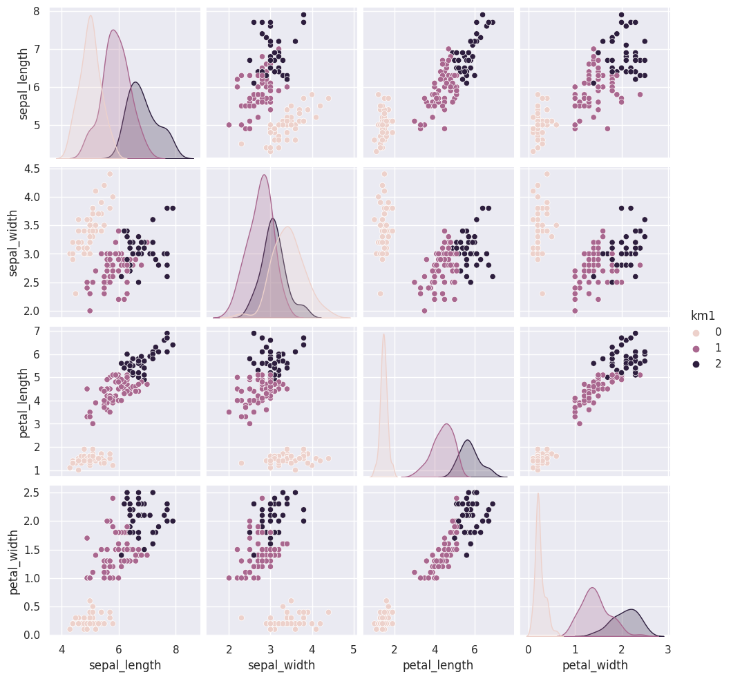
Add the predictions as a new column to the original iris_df and make a pairplot with the points colored by what the clustering learned.
iris_df['km1'] = cluster_assignments
sns.pairplot(data=iris_df, hue='km1')
<seaborn.axisgrid.PairGrid at 0x7fb7504168e0>
We can use the vars parameter to plot only the measurement columns and not the cluster labels. We didn’t have to do this before, because species is strings, so seaborn knows to not plot it, but the cluster predictions are also numerical, so by default seaborn plots them.
iris_df['km3_1'] = cluster_assignments
sns.pairplot(data=iris_df, hue='km3_1', vars=measurement_cols)
<seaborn.axisgrid.PairGrid at 0x7fb74cbfc1f0>

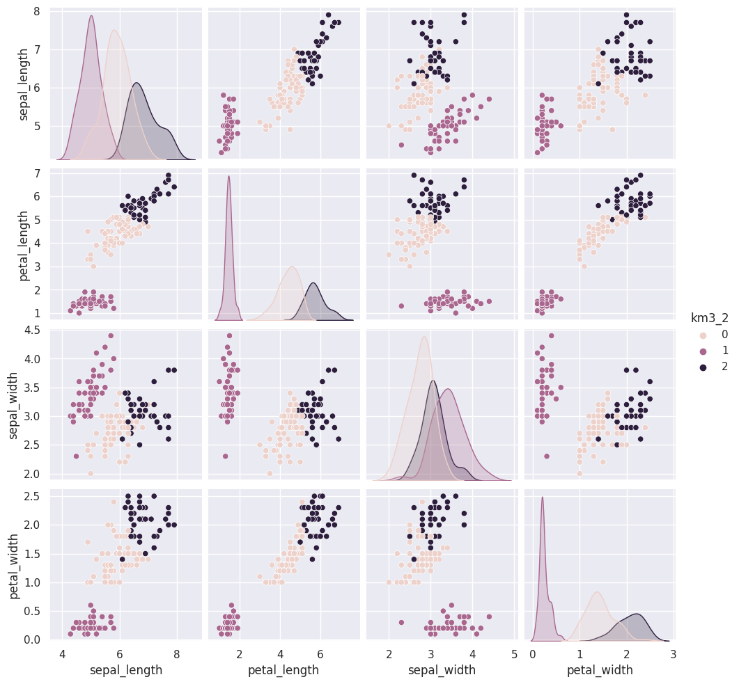
17.4. Clustering Persistence#
We can run kmeans a few more times and plot each time and/or compare with a neighbor/ another group.
iris_df['km3_2'] = km.fit_predict(iris_X)
sns.pairplot(data=iris_df, hue='km3_2', vars=measurement_cols)
/opt/hostedtoolcache/Python/3.8.16/x64/lib/python3.8/site-packages/sklearn/cluster/_kmeans.py:870: FutureWarning: The default value of `n_init` will change from 10 to 'auto' in 1.4. Set the value of `n_init` explicitly to suppress the warning
  warnings.warn(
<seaborn.axisgrid.PairGrid at 0x7fb744fd1e50>
iris_df['km3_3'] = km.fit_predict(iris_X)
sns.pairplot(data=iris_df, hue='km3_3', vars=measurement_cols)
/opt/hostedtoolcache/Python/3.8.16/x64/lib/python3.8/site-packages/sklearn/cluster/_kmeans.py:870: FutureWarning: The default value of `n_init` will change from 10 to 'auto' in 1.4. Set the value of `n_init` explicitly to suppress the warning
  warnings.warn(
<seaborn.axisgrid.PairGrid at 0x7fb743fa8c40>

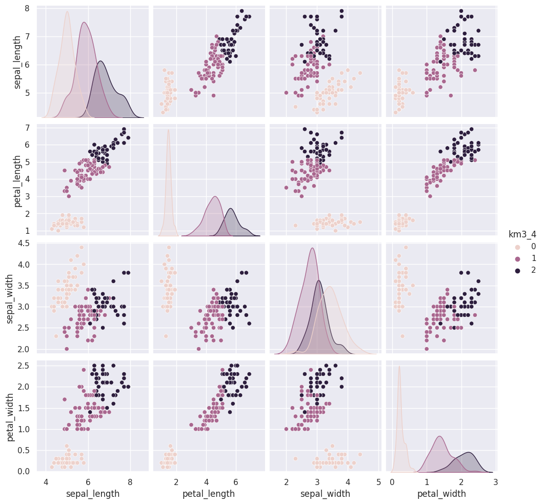
iris_df['km3_4'] = km.fit_predict(iris_X)
sns.pairplot(data=iris_df, hue='km3_4', vars=measurement_cols)
/opt/hostedtoolcache/Python/3.8.16/x64/lib/python3.8/site-packages/sklearn/cluster/_kmeans.py:870: FutureWarning: The default value of `n_init` will change from 10 to 'auto' in 1.4. Set the value of `n_init` explicitly to suppress the warning
  warnings.warn(
<seaborn.axisgrid.PairGrid at 0x7fb743ba84c0>
Note: (do not send this)
give thm time to compare the solutions and ask here.
We could also use a loop (or list comprehension) to repeat kmeans multiple times.
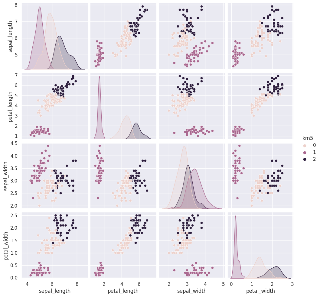
for i in [5,6,7]:
    iris_df['km' + str(i)] = km.fit_predict(iris_X)

sns.pairplot(data=iris_df, hue='km5', vars=measurement_cols)
/opt/hostedtoolcache/Python/3.8.16/x64/lib/python3.8/site-packages/sklearn/cluster/_kmeans.py:870: FutureWarning: The default value of `n_init` will change from 10 to 'auto' in 1.4. Set the value of `n_init` explicitly to suppress the warning
  warnings.warn(
/opt/hostedtoolcache/Python/3.8.16/x64/lib/python3.8/site-packages/sklearn/cluster/_kmeans.py:870: FutureWarning: The default value of `n_init` will change from 10 to 'auto' in 1.4. Set the value of `n_init` explicitly to suppress the warning
  warnings.warn(
/opt/hostedtoolcache/Python/3.8.16/x64/lib/python3.8/site-packages/sklearn/cluster/_kmeans.py:870: FutureWarning: The default value of `n_init` will change from 10 to 'auto' in 1.4. Set the value of `n_init` explicitly to suppress the warning
  warnings.warn(
<seaborn.axisgrid.PairGrid at 0x7fb744008880>
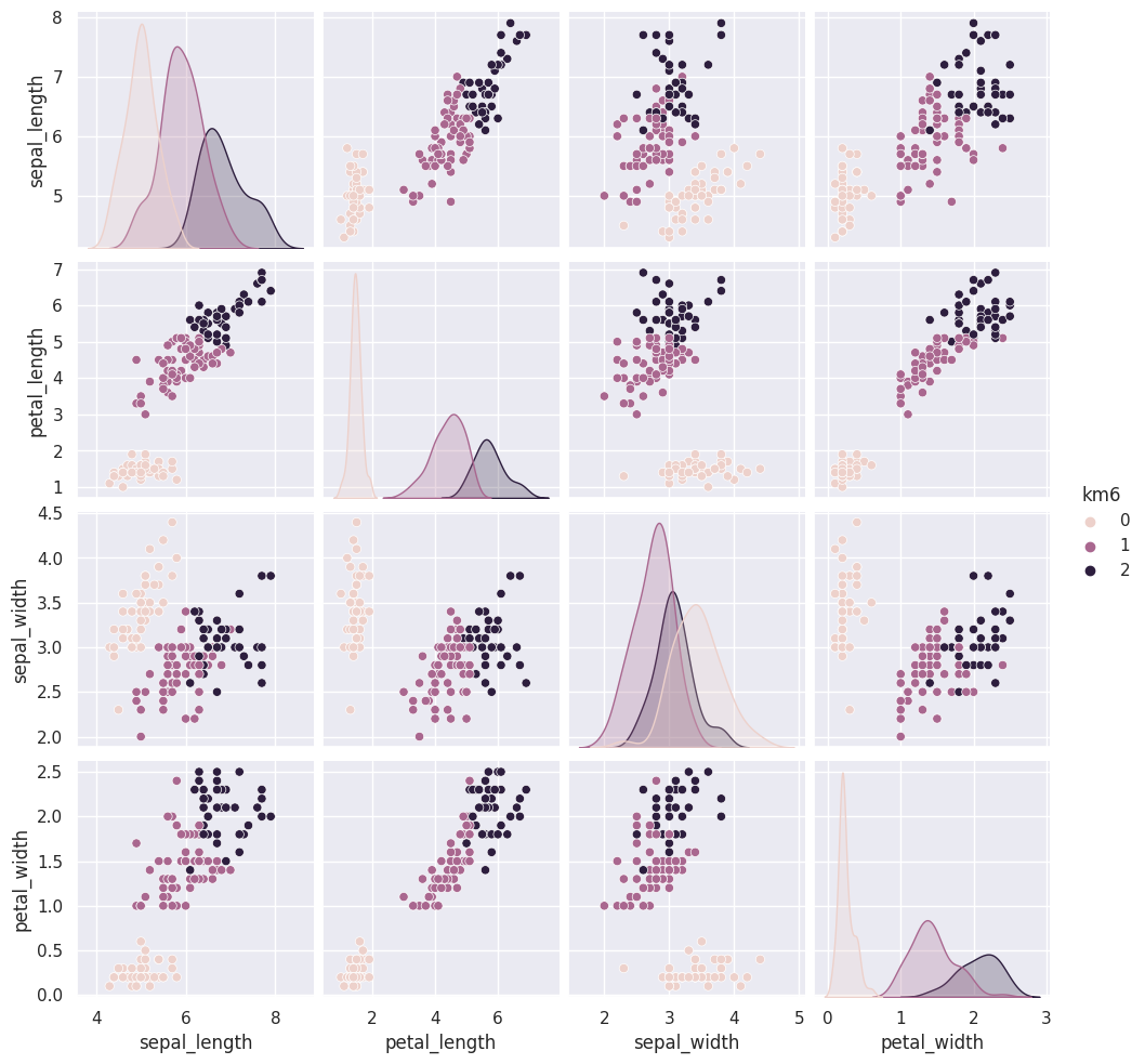
sns.pairplot(data=iris_df, hue='km6', vars=measurement_cols)
<seaborn.axisgrid.PairGrid at 0x7fb742a35310>
sns.pairplot(data=iris_df, hue='km7', vars=measurement_cols)
<seaborn.axisgrid.PairGrid at 0x7fb7422e3eb0>
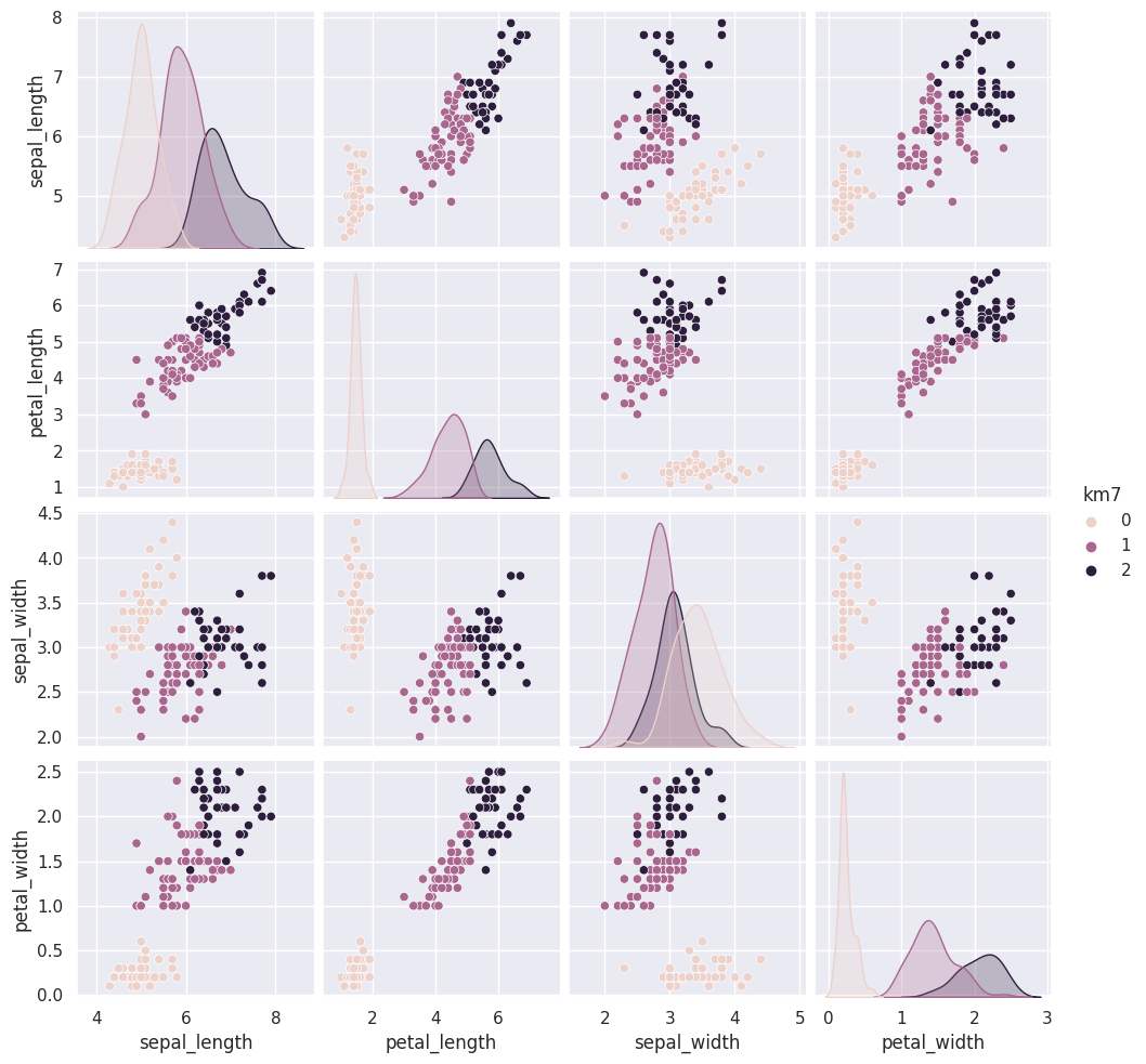
The grouping of the points stay the same across different runs, but which color each group gets assigned to changes. Look at the 5th time compared to the ones before and 6 compared to that. Which blob is which color changes.
Today, we saw that the clustering solution was pretty similar each time in terms of which points were grouped together, but the labeling of the groups (which one was each number) was different each time. We also saw that clustering can only number the clusters, it can’t match them with certainty to the species. This makes evaluating clustering somewhat different, so we need new metrics.
17.5. Clustering Evaluation#
a: The mean distance between a sample and all other points in the same class.
b: The mean distance between a sample and all other points in the next nearest cluster.
This score computes a ratio of how close points are to points in the same cluster vs other clusters
Use the prismia drawing tool (the scribble next to the send button) to draw data (use two colors) that would have a silhouette score of near zero.
(solution is overlapping completely)
Draw clustering solution that would have a silhouette score above
Copmute the Silhouette score for a coupl iteratations and show that thy agree.
iris_df.head()
| sepal_length | sepal_width | petal_length | petal_width | species | km1 | km3_1 | km3_2 | km3_3 | km3_4 | km5 | km6 | km7 | |
|---|---|---|---|---|---|---|---|---|---|---|---|---|---|
| 0 | 5.1 | 3.5 | 1.4 | 0.2 | setosa | 0 | 0 | 1 | 0 | 0 | 1 | 0 | 0 |
| 1 | 4.9 | 3.0 | 1.4 | 0.2 | setosa | 0 | 0 | 1 | 0 | 0 | 1 | 0 | 0 |
| 2 | 4.7 | 3.2 | 1.3 | 0.2 | setosa | 0 | 0 | 1 | 0 | 0 | 1 | 0 | 0 |
| 3 | 4.6 | 3.1 | 1.5 | 0.2 | setosa | 0 | 0 | 1 | 0 | 0 | 1 | 0 | 0 |
| 4 | 5.0 | 3.6 | 1.4 | 0.2 | setosa | 0 | 0 | 1 | 0 | 0 | 1 | 0 | 0 |
metrics.silhouette_score(iris_df[measurement_cols],iris_df['km3_1'])
0.55281901235641
metrics.silhouette_score(iris_df[measurement_cols],iris_df['km3_4'])
0.55281901235641
these are very consistent, but what if we try othr numbers of clustrs
km2 = KMeans(n_clusters=2)
iris_df['km2'] = km2.fit_predict(iris_X)
/opt/hostedtoolcache/Python/3.8.16/x64/lib/python3.8/site-packages/sklearn/cluster/_kmeans.py:870: FutureWarning: The default value of `n_init` will change from 10 to 'auto' in 1.4. Set the value of `n_init` explicitly to suppress the warning
  warnings.warn(
metrics.silhouette_score(iris_df[measurement_cols],iris_df['km2'])
0.6810461692117464
km4 = KMeans(n_clusters=4)
iris_df['km4'] = km4.fit_predict(iris_X)
/opt/hostedtoolcache/Python/3.8.16/x64/lib/python3.8/site-packages/sklearn/cluster/_kmeans.py:870: FutureWarning: The default value of `n_init` will change from 10 to 'auto' in 1.4. Set the value of `n_init` explicitly to suppress the warning
  warnings.warn(
metrics.silhouette_score(iris_df[measurement_cols],iris_df['km4'])
0.4980505049972882
We see now that 2 clusters actually describes this data bettre, even though we were able to clasiify the three species better. This is a common thing to observe.
While we sometims describe things as discrete, in nature a lot of things vary fairly continuously. Clustering works best for things that are truly discrete, but can be useful even when it is not a perfct fit.
17.6. Mutual Information#
When we know the truth, we can see if the learned clusters are related to the true groups, we can’t compare them like accuracy but we can use a metric that is intuitively like a correlation for categorical variables, the mutual information.
The adjusted_mutual_info_score method in the metrics module computes a version of mutual information that is normalized to have good properties. Apply that to the two different clustering solutions and to a solution for K=4.
metrics.adjusted_mutual_info_score(iris_df['species'],iris_df['km3_1'])
0.7551191675800486
metrics.adjusted_mutual_info_score(iris_df['species'],iris_df['km2'])
0.653838071376278
metrics.adjusted_mutual_info_score(iris_df['species'],iris_df['km4'])
0.7172081944051023
Notic here, that the true number is best but adding more clusters makes th MI very similar, If the additional cluster is one of the true ones split, it can still find th original boundaries and so it will still get a high score.
Other types of clustering: sklearn overivew
17.7. Questions#
17.7.1. Is there a way to see all of the seaborn palettes?#
17.7.2. Can you clarify how fit_predict works?#
It is equivalent to calling both the fit and the predict on the same samples.
17.7.3. im very interested in nueral networks i would love to have more lectures on it#
We will!
17.7.4. what types of data is clustering not very useful?#
Groups that are not separate
17.7.5. Was this the formula for \(s = \frac{b-a}{max(a,b)}\) how the silhouette score is computed?#
yes