19. Regression

%matplotlib inline

import numpy as np
import seaborn as sns
import matplotlib.pyplot as plt
from sklearn import datasets, linear_model
from sklearn.metrics import mean_squared_error, r2_score
from sklearn.model_selection import train_test_split
import pandas as pd
sns.set_theme(font_scale=2,palette='colorblind')

tips_df = sns.load_dataset('tips')

tips_df.head()

	total_bill	tip	sex	smoker	day	time	size
0	16.99	1.01	Female	No	Sun	Dinner	2
1	10.34	1.66	Male	No	Sun	Dinner	3
2	21.01	3.50	Male	No	Sun	Dinner	3
3	23.68	3.31	Male	No	Sun	Dinner	2
4	24.59	3.61	Female	No	Sun	Dinner	4

Split the data to use 80% of the data to train a model to predict the tip from the total bill.

tips_X = tips_df['total_bill']
tips_y = tips_df['tip']

type(tips_X.values)

numpy.ndarray

tips_X.values.shape

(244,)

tips_X.values[:,np.newaxis].shape

(244, 1)

tips_X = tips_X.values[:,np.newaxis]
tips_X_train,tips_X_test, tips_y_train, tips_y_test = train_test_split(tips_X, tips_y,
                                                                       train_size=.8)

regr = linear_model.LinearRegression()

type(tips_X)

numpy.ndarray

regr.fit(tips_X_train,tips_y_train)

LinearRegression()

In a Jupyter environment, please rerun this cell to show the HTML representation or trust the notebook.
On GitHub, the HTML representation is unable to render, please try loading this page with nbviewer.org.

regr.get_params()

{'copy_X': True, 'fit_intercept': True, 'n_jobs': None, 'positive': False}

regr.coef_

array([0.10513009])

regr.intercept_

0.8998806720394064

tips_y_pred = regr.predict(tips_X_test)

tips_y_pred[0]

2.7838119316826817

tips_X_test[0]*regr.coef_ + regr.intercept_

array([2.78381193])

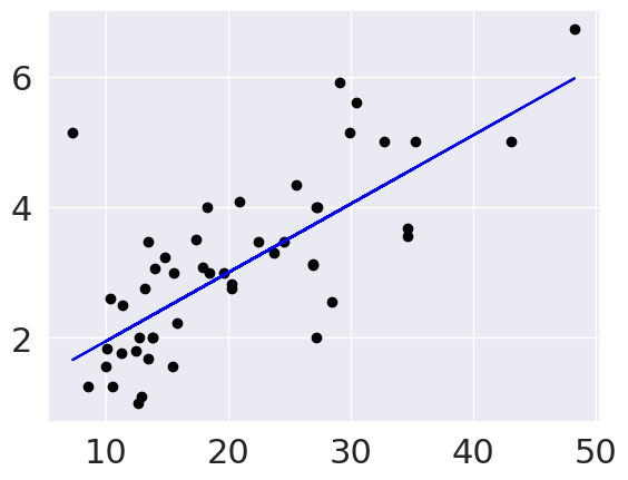
plt.scatter(tips_X_test,tips_y_test, color='black')
plt.plot(tips_X_test,tips_y_pred, color='blue')

[<matplotlib.lines.Line2D at 0x7f8bc9a9df10>]

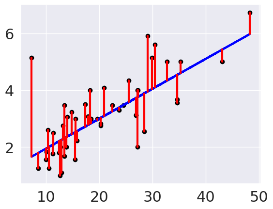
plt.plot(tips_X_test, tips_y_pred, color='blue', linewidth=3)

# draw vertical lines frome each data point to its predict value
[plt.plot([x,x],[yp,yt], color='red', linewidth=3)
                 for x, yp, yt in zip(tips_X_test, tips_y_pred,tips_y_test)];
plt.scatter(tips_X_test, tips_y_test,  color='black')

<matplotlib.collections.PathCollection at 0x7f8bc7961f10>

mean_squared_error(tips_y_test,tips_y_pred)

0.8443482832748362

tips_y_test.mean()

3.1446938775510205

mean_squared_error(tips_y_test,tips_y_pred)/tips_y_test.mean()

0.26849935674259834

r2_score(tips_y_test,tips_y_pred)

0.5218612850368313

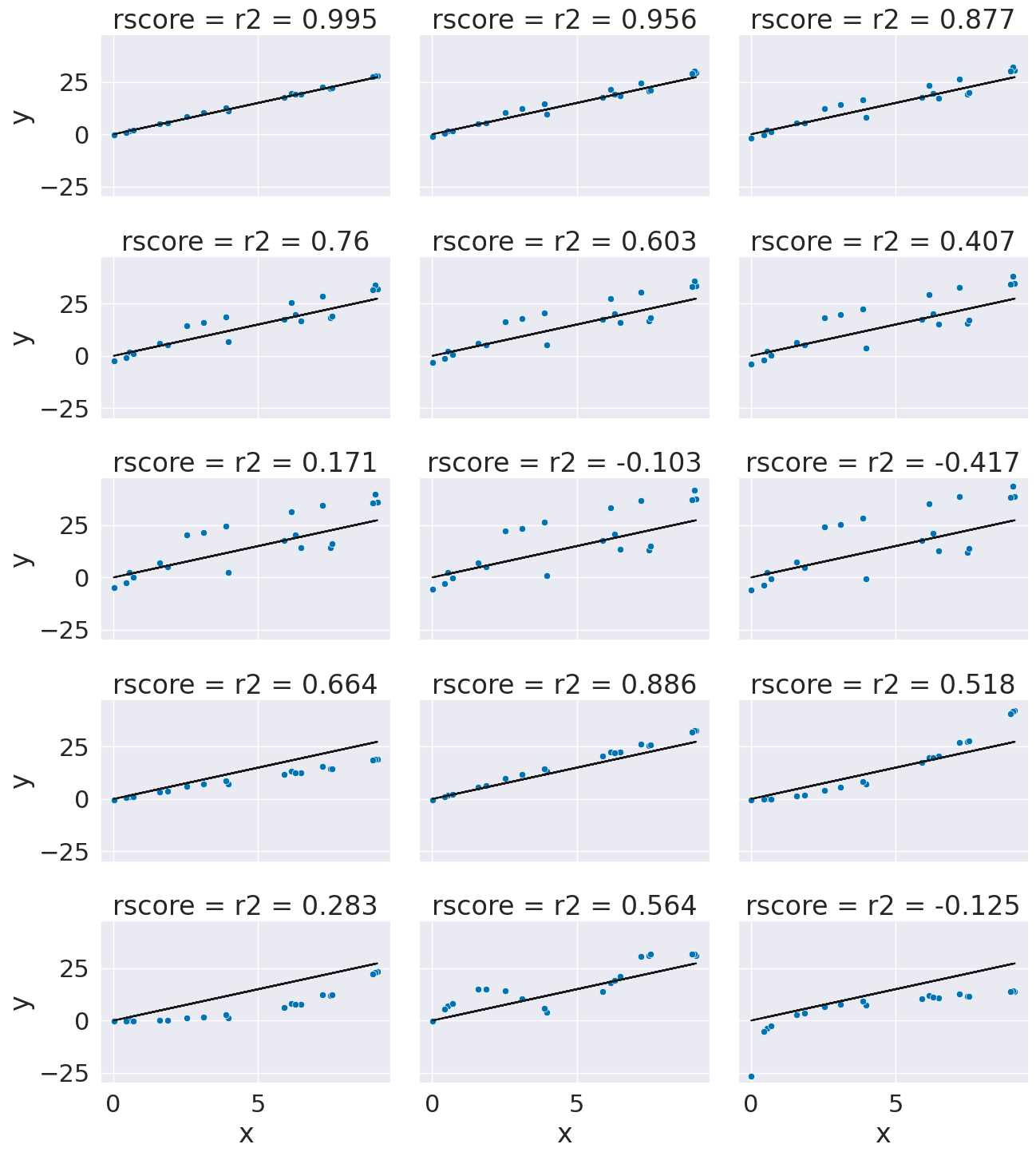
x = 10*np.random.random(20)
y_pred = 3*x
ex_df = pd.DataFrame(data = x,columns = ['x'])
ex_df['y_pred'] = y_pred
n_levels = range(1,18,2)
noise = (np.random.random(20)-.5)*2
for n in n_levels:
    y_true = y_pred + n* noise
    ex_df['r2 = '+ str(np.round(r2_score(y_pred,y_true),3))] = y_true

f_x_list = [2*x,3.5*x,.5*x**2, .03*x**3, 10*np.sin(x)+x*3,3*np.log(x**2)]
for fx in f_x_list:
    y_true = fx + noise
    ex_df['r2 = '+ str(np.round(r2_score(y_pred,y_true),3))] = y_true    

xy_df = ex_df.melt(id_vars=['x','y_pred'],var_name='rscore',value_name='y')
# sns.lmplot(x='x',y='y', data = xy_df,col='rscore',col_wrap=3,)
g = sns.FacetGrid(data = xy_df,col='rscore',col_wrap=3,aspect=1.5,height=3)
g.map(plt.plot, 'x','y_pred',color='k')
g.map(sns.scatterplot, "x", "y",)

<seaborn.axisgrid.FacetGrid at 0x7f8bc791e490>

regr.score(tips_X_test,tips_y_test)

0.5218612850368313

tips_df.head()

	total_bill	tip	sex	smoker	day	time	size
0	16.99	1.01	Female	No	Sun	Dinner	2
1	10.34	1.66	Male	No	Sun	Dinner	3
2	21.01	3.50	Male	No	Sun	Dinner	3
3	23.68	3.31	Male	No	Sun	Dinner	2
4	24.59	3.61	Female	No	Sun	Dinner	4

tips_X2 = tips_df[['total_bill','size']]
tips_X2_train,tips_X2_test, tips_y2_train, tips_y2_test = train_test_split(tips_X2, tips_y,
                                                                       train_size=.8)

regr2 = linear_model.LinearRegression()
regr2.fit(tips_X2_train,tips_y2_train)

LinearRegression()

In a Jupyter environment, please rerun this cell to show the HTML representation or trust the notebook.
On GitHub, the HTML representation is unable to render, please try loading this page with nbviewer.org.

regr2.coef_

array([0.09588457, 0.1885609 ])

regr2.score(tips_X2_test,tips_y2_test)

0.43943140371626077

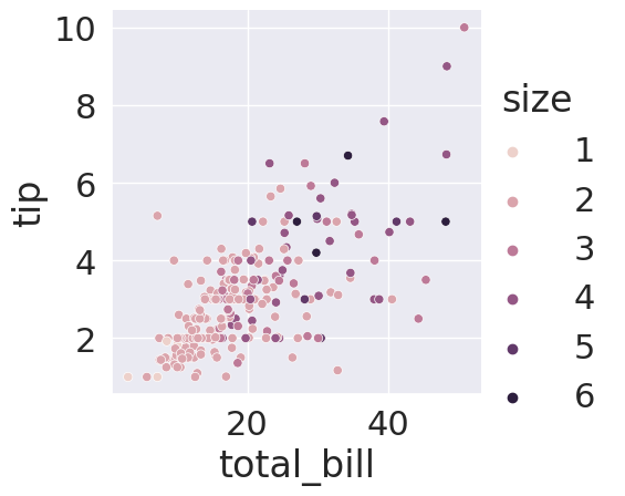
sns.relplot(data=tips_df,x='total_bill',y='tip',
           hue='size')

<seaborn.axisgrid.FacetGrid at 0x7f8bc7916dc0>

from sklearn import datasets

# Load the diabetes dataset
diabetes_X, diabetes_y = datasets.load_diabetes(return_X_y=True)
X_train,X_test, y_train,y_test = train_test_split(diabetes_X, diabetes_y ,
                                                  test_size=20,random_state=0)

regr_db = linear_model.LinearRegression()
regr_db.fit(X_train, y_train)

LinearRegression()

In a Jupyter environment, please rerun this cell to show the HTML representation or trust the notebook.
On GitHub, the HTML representation is unable to render, please try loading this page with nbviewer.org.

y_pred = regr_db.predict(X_test)
r2_score(y_test,y_pred)

0.5195333332288746

diabetes_X.shape

(442, 10)

lasso = linear_model.Lasso()
lasso.fit(X_train, y_train)
lasso.score(X_test,y_test)

0.42249260665177746

lasso = linear_model.Lasso(.5)
lasso.fit(X_train, y_train)
lasso.score(X_test,y_test)

0.527228369284263

lasso = linear_model.Lasso(.25)
lasso.fit(X_train, y_train)
lasso.score(X_test,y_test)

0.5501992246861973

lasso.coef_

array([  -0.        ,  -52.1429064 ,  503.60281992,  219.24141192,
         -0.        ,   -0.        , -147.83111493,    0.        ,
        441.7507385 ,    0.        ])

link to polynomial regression