
22. Model Comparison#
import matplotlib.pyplot as plt
import numpy as np
import seaborn as sns
import pandas as pd
from sklearn import datasets
from sklearn import cluster
from sklearn import svm
from sklearn import tree
# import the whole model selection module
from sklearn import model_selection
sns.set_theme(palette='colorblind')
# load and split the data
iris_X, iris_y = datasets.load_iris(return_X_y=True)
iris_X_train, iris_X_test, iris_y_train, iris_y_test = model_selection.train_test_split(
  iris_X,iris_y, test_size =.2)


# create dt,
dt = tree.DecisionTreeClassifier()

# set param grid
params_dt = {'criterion':['gini','entropy'],
       'max_depth':[2,3,4,5,6],
    'min_samples_leaf':list(range(2,20,2))}
# create optimizer
dt_opt = model_selection.GridSearchCV(dt,params_dt,cv=10)


# optimize the dt parameters
dt_opt.fit(iris_X_train,iris_y_train)

# store the results in a dataframe
dt_df = pd.DataFrame(dt_opt.cv_results_)


# create svm, its parameter grid and optimizer
svm_clf = svm.SVC()
param_grid = {'kernel':['linear','rbf'], 'C':[.5, .75,1,2,5,7, 10]}
svm_opt = model_selection.GridSearchCV(svm_clf,param_grid,cv=10)

# optmize the svm put the CV results in a dataframe
svm_opt.fit(iris_X_train,iris_y_train)
sv_df = pd.DataFrame(svm_opt.cv_results_)
So we have redone some familiar code. We have found the optimal parameters for best accuracy for two different classifiers, SVM and Decision tree on our data.
This is extra detail we did not do in class for time reasons
We can  use EDA to understand how the score varied across all of the parameter settings we tried.

```{code-cell} ipython3
sv_df['mean_test_score'].describe()
dt_df['mean_test_score'].describe()
count    90.000000
mean      0.932963
std       0.004489
min       0.908333
25%       0.933333
50%       0.933333
75%       0.933333
max       0.941667
Name: mean_test_score, dtype: float64
From this we see that in both cases the standard deviation (std) is really low. This tells us that the parameter changes didn’t impact the performance much. Combined with the overall high accuracy this tells us that the data is probably really easy to classify. If the performance had been uniformly bad, it might have instead told us that we did not try a wide enough range of parameters.
To confirm how many parameter settings we have used we can check a couple different ways. First, above in the count of the describe.
We can also calculate directly from the parameter grids before we even do the fit.
description_vars = ['param_C', 'param_kernel', 'params',]
vars_to_plot = ['mean_fit_time', 'std_fit_time', 'mean_score_time', 'std_score_time']
svm_time = sv_df.melt(id_vars= description_vars,
value_vars=vars_to_plot)
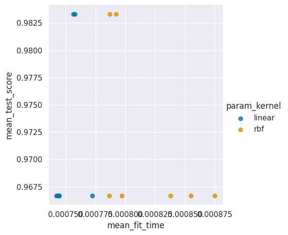
sns.lmplot(data=sv_df, x='mean_fit_time',y='mean_test_score',
hue='param_kernel',fit_reg=False)
<seaborn.axisgrid.FacetGrid at 0x7f821c2d6040>
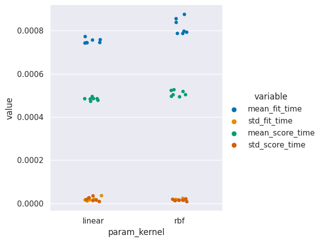
22.1. How does the timing vary?#
Let’s dig in and see which one is better.
sv_df.head(1)
| mean_fit_time | std_fit_time | mean_score_time | std_score_time | param_C | param_kernel | params | split0_test_score | split1_test_score | split2_test_score | split3_test_score | split4_test_score | split5_test_score | split6_test_score | split7_test_score | split8_test_score | split9_test_score | mean_test_score | std_test_score | rank_test_score | |
|---|---|---|---|---|---|---|---|---|---|---|---|---|---|---|---|---|---|---|---|---|
| 0 | 0.000772 | 0.000036 | 0.000495 | 0.000026 | 0.5 | linear | {'C': 0.5, 'kernel': 'linear'} | 0.916667 | 1.0 | 1.0 | 0.916667 | 0.916667 | 1.0 | 1.0 | 0.916667 | 1.0 | 1.0 | 0.966667 | 0.040825 | 5 |
%matplotlib inline
svm_time = sv_df.melt(id_vars=['param_C', 'param_kernel', 'params',],
                      value_vars=['mean_fit_time', 'std_fit_time', 'mean_score_time', 'std_score_time'])
sns.lmplot(data=sv_df, x='mean_fit_time',y='mean_test_score',
          hue='param_kernel',fit_reg=False)
<seaborn.axisgrid.FacetGrid at 0x7f82548b8a30>
svm_time.head()
| param_C | param_kernel | params | variable | value | |
|---|---|---|---|---|---|
| 0 | 0.5 | linear | {'C': 0.5, 'kernel': 'linear'} | mean_fit_time | 0.000772 |
| 1 | 0.5 | rbf | {'C': 0.5, 'kernel': 'rbf'} | mean_fit_time | 0.000875 |
| 2 | 0.75 | linear | {'C': 0.75, 'kernel': 'linear'} | mean_fit_time | 0.000756 |
| 3 | 0.75 | rbf | {'C': 0.75, 'kernel': 'rbf'} | mean_fit_time | 0.000855 |
| 4 | 1 | linear | {'C': 1, 'kernel': 'linear'} | mean_fit_time | 0.000758 |
sns.catplot(data= svm_time, x='param_kernel',y='value',hue='variable')
<seaborn.axisgrid.FacetGrid at 0x7f8219e73df0>
22.2. How does training impact our model?#
Now we can create the learning curve.
train_sizes, train_scores, test_scores, fit_times, score_times = model_selection.learning_curve(svm_opt.best_estimator_,iris_X_train, iris_y_train,
                              train_sizes= [.4,.5,.6,.8],return_times=True)
It returns the list of the counts for each training size (we input percentages and it returns counts)
[train_sizes, train_scores, test_scores, fit_times, score_times]
[array([38, 48, 57, 76]),
 array([[0.97368421, 0.97368421, 0.97368421, 0.97368421, 0.97368421],
        [0.95833333, 0.95833333, 0.95833333, 1.        , 1.        ],
        [0.96491228, 0.98245614, 0.96491228, 0.96491228, 0.96491228],
        [0.98684211, 0.98684211, 0.97368421, 0.96052632, 0.96052632]]),
 array([[0.95833333, 0.95833333, 0.95833333, 0.91666667, 1.        ],
        [0.95833333, 0.95833333, 0.95833333, 0.95833333, 0.95833333],
        [0.95833333, 0.95833333, 0.95833333, 0.95833333, 1.        ],
        [0.95833333, 0.95833333, 0.95833333, 1.        , 1.        ]]),
 array([[0.00085497, 0.00068593, 0.00066113, 0.00065804, 0.00065899],
        [0.00071263, 0.00072145, 0.0007031 , 0.00068736, 0.00068855],
        [0.00072956, 0.00068784, 0.00068784, 0.00069547, 0.00069857],
        [0.00073147, 0.0007441 , 0.00074005, 0.00073743, 0.00073338]]),
 array([[0.00053573, 0.00048327, 0.00047064, 0.00046825, 0.00046372],
        [0.00047469, 0.00047231, 0.00046897, 0.00049663, 0.0004952 ],
        [0.00047112, 0.00046802, 0.00047135, 0.00046992, 0.00046968],
        [0.00047994, 0.00047874, 0.00047636, 0.00050092, 0.00050354]])]
We can use our skills in transforming data to make it easier to exmine just a subset of the scores.
train_scores.mean(axis=1)
array([0.97368421, 0.975 , 0.96842105, 0.97368421])
[train_sizes, train_scores.mean(axis=1), test_scores.mean(axis=1),
                                fit_times.mean(axis=1), score_times.mean(axis=1)]
[array([38, 48, 57, 76]),
 array([0.97368421, 0.975     , 0.96842105, 0.97368421]),
 array([0.95833333, 0.95833333, 0.96666667, 0.975     ]),
 array([0.00070381, 0.00070262, 0.00069985, 0.00073729]),
 array([0.00048432, 0.00048156, 0.00047002, 0.0004879 ])]
np.asarray([train_sizes, train_scores.mean(axis=1), test_scores.mean(axis=1),
                                fit_times.mean(axis=1), score_times.mean(axis=1)]).T
array([[3.80000000e+01, 9.73684211e-01, 9.58333333e-01, 7.03811646e-04,
        4.84323502e-04],
       [4.80000000e+01, 9.75000000e-01, 9.58333333e-01, 7.02619553e-04,
        4.81557846e-04],
       [5.70000000e+01, 9.68421053e-01, 9.66666667e-01, 6.99853897e-04,
        4.70018387e-04],
       [7.60000000e+01, 9.73684211e-01, 9.75000000e-01, 7.37285614e-04,
        4.87899780e-04]])
curve_df = pd.DataFrame(data = np.asarray([train_sizes, train_scores.mean(axis=1), test_scores.mean(axis=1),
                                fit_times.mean(axis=1), score_times.mean(axis=1)]).T,
                    columns = ['train_sizes', 'train_scores', 'test_scores', 'fit_times', 'score_times'])
curve_df.head()
| train_sizes | train_scores | test_scores | fit_times | score_times | |
|---|---|---|---|---|---|
| 0 | 38.0 | 0.973684 | 0.958333 | 0.000704 | 0.000484 |
| 1 | 48.0 | 0.975000 | 0.958333 | 0.000703 | 0.000482 |
| 2 | 57.0 | 0.968421 | 0.966667 | 0.000700 | 0.000470 |
| 3 | 76.0 | 0.973684 | 0.975000 | 0.000737 | 0.000488 |
curve_df_tall = curve_df.melt(id_vars='train_sizes',)
sns.relplot(data =curve_df_tall,x='train_sizes',y ='value',hue ='variable' )
<seaborn.axisgrid.FacetGrid at 0x7f8219ee19a0>
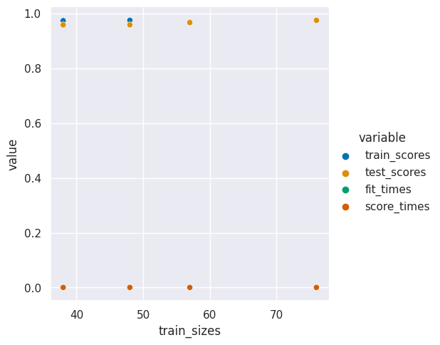
We can see here that the training score and test score are basically the same. This means we’re doing about as well as we cana at learning the a generalizable model and we probably hav enough data for this task.
22.3. When do differences matter?#
We can check calculate a confidence interval to determine more precisely when the performance of two models is meaningfully different.
This function calculates the 95% confidence interval. The range within which we are 95% confident the quantity we have estimated is truly within in. When we have more samples in the test set used to calculate the score, we are more confident in the estimate, so the interval is narrower.
def classification_confint(acc, n):
    '''
    Compute the 95% confidence interval for a classification problem.
      acc -- classification accuracy
      n   -- number of observations used to compute the accuracy
    Returns a tuple (lb,ub)
    '''
    interval = 1.96*np.sqrt(acc*(1-acc)/n)
    lb = max(0, acc - interval)
    ub = min(1.0, acc + interval)
    return (lb,ub)
svm_opt.best_score_, dt_opt.best_score_
(0.9833333333333332, 0.9416666666666668)
We can calculate the number of observations used to compute the accuracy using the size of the training data and the fact that we set it to 10-fold cross validation. That means that 10% (100/10) of the data was used for each fold and each validation set.
150 samples
80% training size (20% test size)
10 fold cross validation
.1*.8*150
12.000000000000002
And thn we can use this to find the range for each model
classification_confint(svm_opt.best_score_,12)
(0.9108997111014602, 1.0)
classification_confint(dt_opt.best_score_,12)
(0.8090578364484199, 1.0)
When the ranges overlap, th models are not significanlty different.
N_diff = 500
classification_confint(svm_opt.best_score_,N_diff), classification_confint(dt_opt.best_score_,N_diff)
((0.9721119648289522, 0.9945547018377141),
 (0.9211229950268541, 0.9622103383064794))
svm_opt.best_estimator_.score(iris_X_test,iris_y_test), dt_opt.best_estimator_.score(iris_X_test,iris_y_test)
(1.0, 1.0)
classification_confint(svm_opt.best_estimator_.score(iris_X_test,iris_y_test),12)
(1.0, 1.0)
classification_confint(dt_opt.best_estimator_.score(iris_X_test,iris_y_test),12)
(1.0, 1.0)
22.4. Digits Dataset#
Today, we’ll load a new dataset and use the default sklearn data structure for datasets. We get back the default data stucture when we use a load_ function without any parameters at all.
digits = datasets.load_digits()
This shows us that the type is defined by sklearn and they called it bunch:
type(digits)
sklearn.utils._bunch.Bunch
We can print it out to begin exploring it.
digits
{'data': array([[ 0.,  0.,  5., ...,  0.,  0.,  0.],
        [ 0.,  0.,  0., ..., 10.,  0.,  0.],
        [ 0.,  0.,  0., ..., 16.,  9.,  0.],
        ...,
        [ 0.,  0.,  1., ...,  6.,  0.,  0.],
        [ 0.,  0.,  2., ..., 12.,  0.,  0.],
        [ 0.,  0., 10., ..., 12.,  1.,  0.]]),
 'target': array([0, 1, 2, ..., 8, 9, 8]),
 'frame': None,
 'feature_names': ['pixel_0_0',
  'pixel_0_1',
  'pixel_0_2',
  'pixel_0_3',
  'pixel_0_4',
  'pixel_0_5',
  'pixel_0_6',
  'pixel_0_7',
  'pixel_1_0',
  'pixel_1_1',
  'pixel_1_2',
  'pixel_1_3',
  'pixel_1_4',
  'pixel_1_5',
  'pixel_1_6',
  'pixel_1_7',
  'pixel_2_0',
  'pixel_2_1',
  'pixel_2_2',
  'pixel_2_3',
  'pixel_2_4',
  'pixel_2_5',
  'pixel_2_6',
  'pixel_2_7',
  'pixel_3_0',
  'pixel_3_1',
  'pixel_3_2',
  'pixel_3_3',
  'pixel_3_4',
  'pixel_3_5',
  'pixel_3_6',
  'pixel_3_7',
  'pixel_4_0',
  'pixel_4_1',
  'pixel_4_2',
  'pixel_4_3',
  'pixel_4_4',
  'pixel_4_5',
  'pixel_4_6',
  'pixel_4_7',
  'pixel_5_0',
  'pixel_5_1',
  'pixel_5_2',
  'pixel_5_3',
  'pixel_5_4',
  'pixel_5_5',
  'pixel_5_6',
  'pixel_5_7',
  'pixel_6_0',
  'pixel_6_1',
  'pixel_6_2',
  'pixel_6_3',
  'pixel_6_4',
  'pixel_6_5',
  'pixel_6_6',
  'pixel_6_7',
  'pixel_7_0',
  'pixel_7_1',
  'pixel_7_2',
  'pixel_7_3',
  'pixel_7_4',
  'pixel_7_5',
  'pixel_7_6',
  'pixel_7_7'],
 'target_names': array([0, 1, 2, 3, 4, 5, 6, 7, 8, 9]),
 'images': array([[[ 0.,  0.,  5., ...,  1.,  0.,  0.],
         [ 0.,  0., 13., ..., 15.,  5.,  0.],
         [ 0.,  3., 15., ..., 11.,  8.,  0.],
         ...,
         [ 0.,  4., 11., ..., 12.,  7.,  0.],
         [ 0.,  2., 14., ..., 12.,  0.,  0.],
         [ 0.,  0.,  6., ...,  0.,  0.,  0.]],

        [[ 0.,  0.,  0., ...,  5.,  0.,  0.],
         [ 0.,  0.,  0., ...,  9.,  0.,  0.],
         [ 0.,  0.,  3., ...,  6.,  0.,  0.],
         ...,
         [ 0.,  0.,  1., ...,  6.,  0.,  0.],
         [ 0.,  0.,  1., ...,  6.,  0.,  0.],
         [ 0.,  0.,  0., ..., 10.,  0.,  0.]],

        [[ 0.,  0.,  0., ..., 12.,  0.,  0.],
         [ 0.,  0.,  3., ..., 14.,  0.,  0.],
         [ 0.,  0.,  8., ..., 16.,  0.,  0.],
         ...,
         [ 0.,  9., 16., ...,  0.,  0.,  0.],
         [ 0.,  3., 13., ..., 11.,  5.,  0.],
         [ 0.,  0.,  0., ..., 16.,  9.,  0.]],

        ...,

        [[ 0.,  0.,  1., ...,  1.,  0.,  0.],
         [ 0.,  0., 13., ...,  2.,  1.,  0.],
         [ 0.,  0., 16., ..., 16.,  5.,  0.],
         ...,
         [ 0.,  0., 16., ..., 15.,  0.,  0.],
         [ 0.,  0., 15., ..., 16.,  0.,  0.],
         [ 0.,  0.,  2., ...,  6.,  0.,  0.]],

        [[ 0.,  0.,  2., ...,  0.,  0.,  0.],
         [ 0.,  0., 14., ..., 15.,  1.,  0.],
         [ 0.,  4., 16., ..., 16.,  7.,  0.],
         ...,
         [ 0.,  0.,  0., ..., 16.,  2.,  0.],
         [ 0.,  0.,  4., ..., 16.,  2.,  0.],
         [ 0.,  0.,  5., ..., 12.,  0.,  0.]],

        [[ 0.,  0., 10., ...,  1.,  0.,  0.],
         [ 0.,  2., 16., ...,  1.,  0.,  0.],
         [ 0.,  0., 15., ..., 15.,  0.,  0.],
         ...,
         [ 0.,  4., 16., ..., 16.,  6.,  0.],
         [ 0.,  8., 16., ..., 16.,  8.,  0.],
         [ 0.,  1.,  8., ..., 12.,  1.,  0.]]]),
 'DESCR': ".. _digits_dataset:\n\nOptical recognition of handwritten digits dataset\n--------------------------------------------------\n\n**Data Set Characteristics:**\n\n    :Number of Instances: 1797\n    :Number of Attributes: 64\n    :Attribute Information: 8x8 image of integer pixels in the range 0..16.\n    :Missing Attribute Values: None\n    :Creator: E. Alpaydin (alpaydin '@' boun.edu.tr)\n    :Date: July; 1998\n\nThis is a copy of the test set of the UCI ML hand-written digits datasets\nhttps://archive.ics.uci.edu/ml/datasets/Optical+Recognition+of+Handwritten+Digits\n\nThe data set contains images of hand-written digits: 10 classes where\neach class refers to a digit.\n\nPreprocessing programs made available by NIST were used to extract\nnormalized bitmaps of handwritten digits from a preprinted form. From a\ntotal of 43 people, 30 contributed to the training set and different 13\nto the test set. 32x32 bitmaps are divided into nonoverlapping blocks of\n4x4 and the number of on pixels are counted in each block. This generates\nan input matrix of 8x8 where each element is an integer in the range\n0..16. This reduces dimensionality and gives invariance to small\ndistortions.\n\nFor info on NIST preprocessing routines, see M. D. Garris, J. L. Blue, G.\nT. Candela, D. L. Dimmick, J. Geist, P. J. Grother, S. A. Janet, and C.\nL. Wilson, NIST Form-Based Handprint Recognition System, NISTIR 5469,\n1994.\n\n.. topic:: References\n\n  - C. Kaynak (1995) Methods of Combining Multiple Classifiers and Their\n    Applications to Handwritten Digit Recognition, MSc Thesis, Institute of\n    Graduate Studies in Science and Engineering, Bogazici University.\n  - E. Alpaydin, C. Kaynak (1998) Cascading Classifiers, Kybernetika.\n  - Ken Tang and Ponnuthurai N. Suganthan and Xi Yao and A. Kai Qin.\n    Linear dimensionalityreduction using relevance weighted LDA. School of\n    Electrical and Electronic Engineering Nanyang Technological University.\n    2005.\n  - Claudio Gentile. A New Approximate Maximal Margin Classification\n    Algorithm. NIPS. 2000.\n"}
We note that it has key value pairs, and that the last one is called DESCR and is text that describes the data. If we send that to the print function it will be formatted more readably.
print(digits['DESCR'])
.. _digits_dataset:

Optical recognition of handwritten digits dataset
--------------------------------------------------

**Data Set Characteristics:**

    :Number of Instances: 1797
    :Number of Attributes: 64
    :Attribute Information: 8x8 image of integer pixels in the range 0..16.
    :Missing Attribute Values: None
    :Creator: E. Alpaydin (alpaydin '@' boun.edu.tr)
    :Date: July; 1998

This is a copy of the test set of the UCI ML hand-written digits datasets
https://archive.ics.uci.edu/ml/datasets/Optical+Recognition+of+Handwritten+Digits

The data set contains images of hand-written digits: 10 classes where
each class refers to a digit.

Preprocessing programs made available by NIST were used to extract
normalized bitmaps of handwritten digits from a preprinted form. From a
total of 43 people, 30 contributed to the training set and different 13
to the test set. 32x32 bitmaps are divided into nonoverlapping blocks of
4x4 and the number of on pixels are counted in each block. This generates
an input matrix of 8x8 where each element is an integer in the range
0..16. This reduces dimensionality and gives invariance to small
distortions.

For info on NIST preprocessing routines, see M. D. Garris, J. L. Blue, G.
T. Candela, D. L. Dimmick, J. Geist, P. J. Grother, S. A. Janet, and C.
L. Wilson, NIST Form-Based Handprint Recognition System, NISTIR 5469,
1994.

.. topic:: References

  - C. Kaynak (1995) Methods of Combining Multiple Classifiers and Their
    Applications to Handwritten Digit Recognition, MSc Thesis, Institute of
    Graduate Studies in Science and Engineering, Bogazici University.
  - E. Alpaydin, C. Kaynak (1998) Cascading Classifiers, Kybernetika.
  - Ken Tang and Ponnuthurai N. Suganthan and Xi Yao and A. Kai Qin.
    Linear dimensionalityreduction using relevance weighted LDA. School of
    Electrical and Electronic Engineering Nanyang Technological University.
    2005.
  - Claudio Gentile. A New Approximate Maximal Margin Classification
    Algorithm. NIPS. 2000.
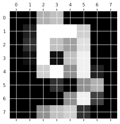
This tells us that we are going to be predicting what digit (0,1,2,3,4,5,6,7,8, or 9) is in the image.
To get an idea of what the images look like, we can use matshow which is short for matrix show. It takes a 2D matrix and plots it as a grayscale image. To get the actual color bar, we use the matplotlib plt.gray().
plt.gray()
plt.matshow(digits.images[9])
<matplotlib.image.AxesImage at 0x7f8219c84a90>
<Figure size 640x480 with 0 Axes>
For easier ML, we will reload it differently:
digits_X, digits_y = datasets.load_digits(return_X_y=True)
This has one row for each sample and has reshaped the 8x8 image into a 64 length vector. So we have one ‘feature’ for each pixel in the images.
digits_X.shape
(1797, 64)
Now we can train a model and generate a learning curve.
svm_clf_digits = svm.SVC()
train_sizes, train_scores, test_scores, fit_times, score_times = model_selection.learning_curve(
                            svm_clf_digits,digits_X, digits_y,
                              train_sizes= [.4,.5,.6,.8,.9, .95],return_times=True)
digits_curve_df = pd.DataFrame(data = np.asarray([train_sizes, train_scores.mean(axis=1), test_scores.mean(axis=1),
                                fit_times.mean(axis=1), score_times.mean(axis=1)]).T,
                    columns = ['train_sizes', 'train_scores', 'test_scores', 'fit_times', 'score_times'])
digits_curve_df_tall = digits_curve_df.melt(id_vars = 'train_sizes', value_vars=[ 'train_scores', 'test_scores'])
sns.relplot(data =digits_curve_df_tall, x = 'train_sizes',y='value',hue='variable',)
<seaborn.axisgrid.FacetGrid at 0x7f8219c76520>
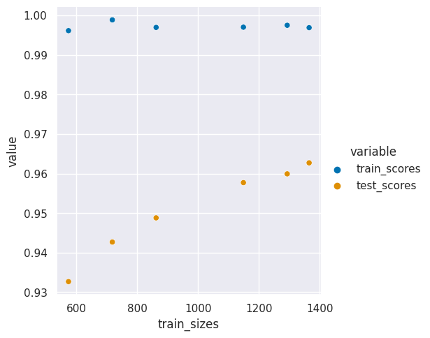
This larger gap shows that a different model or maybe more data could help us learn better. Th good news is that we are probably not overfitting, overfitting would occur when the training accuracy still improves but the test accuracy goes down.