Class 6: Exploratory Data Analysis¶

Warmup¶

topics = ['what is data science', 'jupyter', 'conditional','functions', 'lists', 'dictionaries','pandas' ]
topics

['what is data science',
 'jupyter',
 'conditional',
 'functions',
 'lists',
 'dictionaries',
 'pandas']

What happens when we index with -1?

topics[-1]

'pandas'

We get the last value.

Recall last class we used : to index DataFrames with .loc, we can do that with lists too:

topics[-2:]

['dictionaries', 'pandas']

Announcements¶

next assignment will go up today
try practingin throughout the week
Check Brightspace for TA office hours

Why Exploratory Data Analysis (EDA) before cleaning?¶

Typically a Data process looks like one of these figures:

dsprocess osem

ds process roles

Data cleaning, which some of you asked about on Friday, would typically, happen before EDA, but it’s hard to know what good data looks like, until you’re used to manipulating it. Also, it’s hard to check if data is good (and your cleaning worked) without some EDA. So, I’m choosing to teach EDA first. We’ll do data cleaning next, with these tools from EDA available as options for checking and determining what cleaning to do.

EDA¶

# a version of the SAFI data with more columns
data_url = 'https://raw.githubusercontent.com/brownsarahm/python-socialsci-files/master/data/SAFI_full_shortname.csv'

As usual, we import pandas

import pandas as pd

and pull in the data.

safi_df = pd.read_csv(data_url)
safi_df.head(2)

	key_id	interview_date	quest_no	start	end	province	district	ward	village	years_farm	...	items_owned	items_owned_other	no_meals	months_lack_food	no_food_mitigation	gps_Latitude	gps_Longitude	gps_Altitude	gps_Accuracy	instanceID
0	1	17 November 2016	1	2017-03-23T09:49:57.000Z	2017-04-02T17:29:08.000Z	Manica	Manica	Bandula	God	11	...	['bicycle' ; 'television' ; 'solar_panel' ; ...	NaN	2	['Jan']	['na' ; 'rely_less_food' ; 'reduce_meals' ; ...	-19.112259	33.483456	698	14.0	uuid:ec241f2c-0609-46ed-b5e8-fe575f6cefef
1	2	17 November 2016	1	2017-04-02T09:48:16.000Z	2017-04-02T17:26:19.000Z	Manica	Manica	Bandula	God	2	...	['cow_cart' ; 'bicycle' ; 'radio' ; 'cow_pl...	NaN	2	['Jan' ; 'Sept' ; 'Oct' ; 'Nov' ; 'Dec']	['na' ; 'reduce_meals' ; 'restrict_adults' ;...	-19.112477	33.483416	690	19.0	uuid:099de9c9-3e5e-427b-8452-26250e840d6e

2 rows × 65 columns

Recall on Friday, we can use describe to see several common descriptive statistics

safi_df.describe()

	key_id	quest_no	years_farm	note2	no_membrs	members_count	years_liv	respondent_wall_type_other	buildings_in_compound	rooms	...	note	money_source_other	liv_owned_other	liv_count	items_owned_other	no_meals	gps_Latitude	gps_Longitude	gps_Altitude	gps_Accuracy
count	131.000000	131.000000	131.000000	0.0	131.00000	131.00000	131.000000	0.0	131.000000	131.000000	...	0.0	0.0	0.0	131.000000	0.0	131.000000	131.000000	131.000000	131.000000	131.000000
mean	66.000000	85.473282	15.832061	NaN	7.19084	7.19084	23.053435	NaN	2.068702	1.740458	...	NaN	NaN	NaN	2.366412	NaN	2.603053	-19.102671	33.471971	648.221374	71.115344
std	37.960506	63.151628	10.903883	NaN	3.17227	3.17227	16.913041	NaN	1.241530	1.092547	...	NaN	NaN	NaN	1.082775	NaN	0.491143	0.023754	0.027081	187.697067	335.854190
min	1.000000	1.000000	1.000000	NaN	2.00000	2.00000	1.000000	NaN	1.000000	1.000000	...	NaN	NaN	NaN	1.000000	NaN	2.000000	-19.114989	33.403836	0.000000	3.000000
25%	33.500000	32.500000	8.000000	NaN	5.00000	5.00000	12.000000	NaN	1.000000	1.000000	...	NaN	NaN	NaN	1.000000	NaN	2.000000	-19.112222	33.483329	691.000000	9.000000
50%	66.000000	66.000000	15.000000	NaN	7.00000	7.00000	20.000000	NaN	2.000000	1.000000	...	NaN	NaN	NaN	2.000000	NaN	3.000000	-19.112188	33.483397	702.000000	11.000000
75%	98.500000	138.000000	20.500000	NaN	9.00000	9.00000	27.500000	NaN	3.000000	2.000000	...	NaN	NaN	NaN	3.000000	NaN	3.000000	-19.112077	33.483438	710.000000	13.000000
max	131.000000	202.000000	60.000000	NaN	19.00000	19.00000	96.000000	NaN	8.000000	8.000000	...	NaN	NaN	NaN	5.000000	NaN	3.000000	-19.042909	33.488268	745.000000	2099.999000

8 rows × 25 columns

Then we remember that this includes key_id as a variable tht we don’t actually want to treat as a variable, it’s an index. We can change that with set_index and we can do it in memory (without assignment) using the inplace keyword.

safi_df.set_index('key_id',inplace=True)
safi_df.describe()

	quest_no	years_farm	note2	no_membrs	members_count	years_liv	respondent_wall_type_other	buildings_in_compound	rooms	no_plots	...	note	money_source_other	liv_owned_other	liv_count	items_owned_other	no_meals	gps_Latitude	gps_Longitude	gps_Altitude	gps_Accuracy
count	131.000000	131.000000	0.0	131.00000	131.00000	131.000000	0.0	131.000000	131.000000	131.000000	...	0.0	0.0	0.0	131.000000	0.0	131.000000	131.000000	131.000000	131.000000	131.000000
mean	85.473282	15.832061	NaN	7.19084	7.19084	23.053435	NaN	2.068702	1.740458	2.229008	...	NaN	NaN	NaN	2.366412	NaN	2.603053	-19.102671	33.471971	648.221374	71.115344
std	63.151628	10.903883	NaN	3.17227	3.17227	16.913041	NaN	1.241530	1.092547	1.078210	...	NaN	NaN	NaN	1.082775	NaN	0.491143	0.023754	0.027081	187.697067	335.854190
min	1.000000	1.000000	NaN	2.00000	2.00000	1.000000	NaN	1.000000	1.000000	1.000000	...	NaN	NaN	NaN	1.000000	NaN	2.000000	-19.114989	33.403836	0.000000	3.000000
25%	32.500000	8.000000	NaN	5.00000	5.00000	12.000000	NaN	1.000000	1.000000	2.000000	...	NaN	NaN	NaN	1.000000	NaN	2.000000	-19.112222	33.483329	691.000000	9.000000
50%	66.000000	15.000000	NaN	7.00000	7.00000	20.000000	NaN	2.000000	1.000000	2.000000	...	NaN	NaN	NaN	2.000000	NaN	3.000000	-19.112188	33.483397	702.000000	11.000000
75%	138.000000	20.500000	NaN	9.00000	9.00000	27.500000	NaN	3.000000	2.000000	3.000000	...	NaN	NaN	NaN	3.000000	NaN	3.000000	-19.112077	33.483438	710.000000	13.000000
max	202.000000	60.000000	NaN	19.00000	19.00000	96.000000	NaN	8.000000	8.000000	8.000000	...	NaN	NaN	NaN	5.000000	NaN	3.000000	-19.042909	33.488268	745.000000	2099.999000

8 rows × 24 columns

Try it yourself!

You can use settings on pd.read_csv to set the index when the data is read in instead of doing this after the fact

We can also use the descriptive statistics on a single variable.

safi_df['years_farm'].describe()

count    131.000000
mean      15.832061
std       10.903883
min        1.000000
25%        8.000000
50%       15.000000
75%       20.500000
max       60.000000
Name: years_farm, dtype: float64

Note however that this is not well formatted, that’s because it’s a Series instead of a DataFrame

type(safi_df['years_farm'].describe())

pandas.core.series.Series

We can use reset_index() to make it back into a dataframe

safi_df['years_farm'].describe().reset_index()

	index	years_farm
0	count	131.000000
1	mean	15.832061
2	std	10.903883
3	min	1.000000
4	25%	8.000000
5	50%	15.000000
6	75%	20.500000
7	max	60.000000

And we can drop the added index:

safi_df['years_farm'].describe().reset_index().set_index('index')

	years_farm
index
count	131.000000
mean	15.832061
std	10.903883
min	1.000000
25%	8.000000
50%	15.000000
75%	20.500000
max	60.000000

Note

See that we can chain operations together. This is a helpful feature, but to be used with care. Pep8, the style conventions for python, recommends no more than 79 characters per line. A summary and another summary

We can also use individual summary statistics on DataFrame or Series objects

safi_df['no_membrs'].max()

Split - Apply - Combine¶

A powerful tool in pandas (and data analysis in general) is the ability to apply functions to subsets of the data.

split-apply-combine

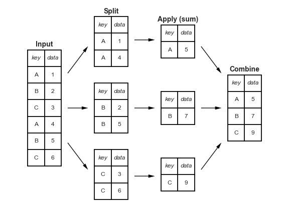
For example, we can get descriptive statistics per village

safi_df.groupby('village').describe()

	quest_no								years_farm		...	gps_Altitude		gps_Accuracy
	count	mean	std	min	25%	50%	75%	max	count	mean	...	75%	max	count	mean	std	min	25%	50%	75%	max
village
Chirodzo	39.0	62.487179	44.261705	8.0	44.5	55.0	64.5	200.0	39.0	17.282051	...	710.0	733.0	39.0	12.461538	7.089080	4.0	9.0	11.0	12.0	39.000
God	43.0	81.720930	77.863839	1.0	14.5	40.0	168.5	202.0	43.0	14.883721	...	709.5	722.0	43.0	12.630512	6.075239	4.0	9.0	11.0	13.5	30.000
Ruaca	49.0	107.061224	55.024013	23.0	72.0	113.0	152.0	194.0	49.0	15.510204	...	711.0	745.0	49.0	169.122408	538.291474	3.0	6.0	9.0	12.0	2099.999

3 rows × 192 columns

We can also rearrange this into a more usable format than this very wide format:

safi_df.groupby('village').describe().unstack().reset_index()

	level_0	level_1	village	0
0	quest_no	count	Chirodzo	39.000000
1	quest_no	count	God	43.000000
2	quest_no	count	Ruaca	49.000000
3	quest_no	mean	Chirodzo	62.487179
4	quest_no	mean	God	81.720930
...	...	...	...	...
571	gps_Accuracy	75%	God	13.500000
572	gps_Accuracy	75%	Ruaca	12.000000
573	gps_Accuracy	max	Chirodzo	39.000000
574	gps_Accuracy	max	God	30.000000
575	gps_Accuracy	max	Ruaca	2099.999000

576 rows × 4 columns

This, however, gives some funny variable names, to fix that, we first save it to a variable.

village_summary_df = safi_df.groupby('village').describe().unstack().reset_index()

Now we can use the rename function

help(village_summary_df.rename)

Help on method rename in module pandas.core.frame:

rename(mapper=None, index=None, columns=None, axis=None, copy=True, inplace=False, level=None, errors='ignore') method of pandas.core.frame.DataFrame instance
    Alter axes labels.
    
    Function / dict values must be unique (1-to-1). Labels not contained in
    a dict / Series will be left as-is. Extra labels listed don't throw an
    error.
    
    See the :ref:`user guide <basics.rename>` for more.
    
    Parameters
    ----------
    mapper : dict-like or function
        Dict-like or function transformations to apply to
        that axis' values. Use either ``mapper`` and ``axis`` to
        specify the axis to target with ``mapper``, or ``index`` and
        ``columns``.
    index : dict-like or function
        Alternative to specifying axis (``mapper, axis=0``
        is equivalent to ``index=mapper``).
    columns : dict-like or function
        Alternative to specifying axis (``mapper, axis=1``
        is equivalent to ``columns=mapper``).
    axis : {0 or 'index', 1 or 'columns'}, default 0
        Axis to target with ``mapper``. Can be either the axis name
        ('index', 'columns') or number (0, 1). The default is 'index'.
    copy : bool, default True
        Also copy underlying data.
    inplace : bool, default False
        Whether to return a new DataFrame. If True then value of copy is
        ignored.
    level : int or level name, default None
        In case of a MultiIndex, only rename labels in the specified
        level.
    errors : {'ignore', 'raise'}, default 'ignore'
        If 'raise', raise a `KeyError` when a dict-like `mapper`, `index`,
        or `columns` contains labels that are not present in the Index
        being transformed.
        If 'ignore', existing keys will be renamed and extra keys will be
        ignored.
    
    Returns
    -------
    DataFrame or None
        DataFrame with the renamed axis labels or None if ``inplace=True``.
    
    Raises
    ------
    KeyError
        If any of the labels is not found in the selected axis and
        "errors='raise'".
    
    See Also
    --------
    DataFrame.rename_axis : Set the name of the axis.
    
    Examples
    --------
    ``DataFrame.rename`` supports two calling conventions
    
    * ``(index=index_mapper, columns=columns_mapper, ...)``
    * ``(mapper, axis={'index', 'columns'}, ...)``
    
    We *highly* recommend using keyword arguments to clarify your
    intent.
    
    Rename columns using a mapping:
    
    >>> df = pd.DataFrame({"A": [1, 2, 3], "B": [4, 5, 6]})
    >>> df.rename(columns={"A": "a", "B": "c"})
       a  c
    0  1  4
    1  2  5
    2  3  6
    
    Rename index using a mapping:
    
    >>> df.rename(index={0: "x", 1: "y", 2: "z"})
       A  B
    x  1  4
    y  2  5
    z  3  6
    
    Cast index labels to a different type:
    
    >>> df.index
    RangeIndex(start=0, stop=3, step=1)
    >>> df.rename(index=str).index
    Index(['0', '1', '2'], dtype='object')
    
    >>> df.rename(columns={"A": "a", "B": "b", "C": "c"}, errors="raise")
    Traceback (most recent call last):
    KeyError: ['C'] not found in axis
    
    Using axis-style parameters:
    
    >>> df.rename(str.lower, axis='columns')
       a  b
    0  1  4
    1  2  5
    2  3  6
    
    >>> df.rename({1: 2, 2: 4}, axis='index')
       A  B
    0  1  4
    2  2  5
    4  3  6

Rename takes a dict-like or function that maps from what’s there to what to change it to. We can either provide the mapper and an axis or pass the mapper as the columns parameter. The columns parameter makes it more human readable, and explicit what we’re doing.

renaming_dict = {'level_0':'variable',
                'level_1':'statistic',
                0:'value'}
village_summary_df.rename(columns= renaming_dict,inplace=True)

Now we have a much better summary table. This is in what’s called tidy format. Each colum

village_summary_df.head()

	variable	statistic	village	value
0	quest_no	count	Chirodzo	39.000000
1	quest_no	count	God	43.000000
2	quest_no	count	Ruaca	49.000000
3	quest_no	mean	Chirodzo	62.487179
4	quest_no	mean	God	81.720930

How could we use this to compute the average across villages for each statistic of each variable?

Try it yourself!

What would it look like to do this from the first result of describe() on the groupby, instead of with the unstack and reset_index?

We do need to groupby 'statistic' and use mean, but that’s not enough:

village_summary_df.groupby('statistic').mean()

	value
statistic
25%	44.807522
50%	48.428030
75%	54.062308
count	30.388889
max	105.468983
mean	49.868824
min	13.756913
std	24.588967

This averages across all of the variables, too. So instead we need to groupby two variables.

village_summary_df.groupby(['statistic','variable']).mean()

		value
statistic	variable
25%	buildings_in_compound	1.000000
	gps_Accuracy	8.000000
	gps_Altitude	691.833333
	gps_Latitude	-19.112221
	gps_Longitude	33.480944
...	...	...
std	respondent_wall_type_other	NaN
	rooms	1.082409
	years_farm	10.832121
	years_liv	16.549343
	yes_group_count	1.074600

192 rows × 1 columns

safi_df.columns

Index(['interview_date', 'quest_no', 'start', 'end', 'province', 'district',
       'ward', 'village', 'years_farm', 'agr_assoc', 'note2', 'no_membrs',
       'members_count', 'remittance_money', 'years_liv', 'parents_liv',
       'sp_parents_liv', 'grand_liv', 'sp_grand_liv', 'respondent_roof_type',
       'respondent_wall_type', 'respondent_wall_type_other',
       'respondent_floor_type', 'window_type', 'buildings_in_compound',
       'rooms', 'other_buildings', 'no_plots', 'plots_count', 'water_use',
       'no_group_count', 'yes_group_count', 'no_enough_water',
       'months_no_water', 'period_use', 'exper_other', 'other_meth',
       'res_change', 'memb_assoc', 'resp_assoc', 'fees_water',
       'affect_conflicts', 'note', 'need_money', 'money_source',
       'money_source_other', 'crops_contr', 'emply_lab', 'du_labour',
       'liv_owned', 'liv_owned_other', 'liv_count', 'poultry',
       'du_look_aftr_cows', 'items_owned', 'items_owned_other', 'no_meals',
       'months_lack_food', 'no_food_mitigation', 'gps_Latitude',
       'gps_Longitude', 'gps_Altitude', 'gps_Accuracy', 'instanceID'],
      dtype='object')

What is the most common combination of respondent_wall_type and respondent_floor_type?

safi_df.groupby(['respondent_wall_type','respondent_floor_type'])['instanceID'].count().reset_index()

	respondent_wall_type	respondent_floor_type	instanceID
0	burntbricks	cement	30
1	burntbricks	earth	37
2	cement	cement	1
3	muddaub	cement	3
4	muddaub	earth	43
5	sunbricks	cement	4
6	sunbricks	earth	13

We can read this table to see the result. Or we might want it in a different way

safi_df.groupby(['respondent_wall_type','respondent_floor_type'])['instanceID'].count().unstack()

respondent_floor_type	cement	earth
respondent_wall_type
burntbricks	30.0	37.0
cement	1.0	NaN
muddaub	3.0	43.0
sunbricks	4.0	13.0

Questions After Class¶

What does the inplace parameter do?¶

We used inplace for the first time today right after we read in the data. Let’s make a new DataFrame and compare what happens with and without.

safi_df_noinplace = pd.read_csv(data_url)
safi_df_inplace = pd.read_csv(data_url)

type(safi_df_noinplace.set_index('key_id'))

pandas.core.frame.DataFrame

safi_df_noinplace.head()

	key_id	interview_date	quest_no	start	end	province	district	ward	village	years_farm	...	items_owned	items_owned_other	no_meals	months_lack_food	no_food_mitigation	gps_Latitude	gps_Longitude	gps_Altitude	gps_Accuracy	instanceID
0	1	17 November 2016	1	2017-03-23T09:49:57.000Z	2017-04-02T17:29:08.000Z	Manica	Manica	Bandula	God	11	...	['bicycle' ; 'television' ; 'solar_panel' ; ...	NaN	2	['Jan']	['na' ; 'rely_less_food' ; 'reduce_meals' ; ...	-19.112259	33.483456	698	14.0	uuid:ec241f2c-0609-46ed-b5e8-fe575f6cefef
1	2	17 November 2016	1	2017-04-02T09:48:16.000Z	2017-04-02T17:26:19.000Z	Manica	Manica	Bandula	God	2	...	['cow_cart' ; 'bicycle' ; 'radio' ; 'cow_pl...	NaN	2	['Jan' ; 'Sept' ; 'Oct' ; 'Nov' ; 'Dec']	['na' ; 'reduce_meals' ; 'restrict_adults' ;...	-19.112477	33.483416	690	19.0	uuid:099de9c9-3e5e-427b-8452-26250e840d6e
2	3	17 November 2016	3	2017-04-02T14:35:26.000Z	2017-04-02T17:26:53.000Z	Manica	Manica	Bandula	God	40	...	['solar_torch']	NaN	2	['Jan' ; 'Feb' ; 'Mar' ; 'Oct' ; 'Nov' ; ...	['na' ; 'restrict_adults' ; 'lab_ex_food']	-19.112108	33.483450	674	13.0	uuid:193d7daf-9582-409b-bf09-027dd36f9007
3	4	17 November 2016	4	2017-04-02T14:55:18.000Z	2017-04-02T17:27:16.000Z	Manica	Manica	Bandula	God	6	...	['bicycle' ; 'radio' ; 'cow_plough' ; 'sola...	NaN	2	['Sept' ; 'Oct' ; 'Nov' ; 'Dec']	['na' ; 'reduce_meals' ; 'restrict_adults' ;...	-19.112229	33.483424	679	5.0	uuid:148d1105-778a-4755-aa71-281eadd4a973
4	5	17 November 2016	5	2017-04-02T15:10:35.000Z	2017-04-02T17:27:35.000Z	Manica	Manica	Bandula	God	18	...	['motorcyle' ; 'radio' ; 'cow_plough' ; 'mo...	NaN	2	['Aug' ; 'Sept' ; 'Oct' ; 'Nov']	['na' ; 'go_forest' ; 'migrate']	-19.112217	33.483425	689	10.0	uuid:2c867811-9696-4966-9866-f35c3e97d02d

5 rows × 65 columns

type(safi_df_inplace.set_index('key_id',inplace=True))

NoneType

safi_df_inplace.head()

	interview_date	quest_no	start	end	province	district	ward	village	years_farm	agr_assoc	...	items_owned	items_owned_other	no_meals	months_lack_food	no_food_mitigation	gps_Latitude	gps_Longitude	gps_Altitude	gps_Accuracy	instanceID
key_id
1	17 November 2016	1	2017-03-23T09:49:57.000Z	2017-04-02T17:29:08.000Z	Manica	Manica	Bandula	God	11	no	...	['bicycle' ; 'television' ; 'solar_panel' ; ...	NaN	2	['Jan']	['na' ; 'rely_less_food' ; 'reduce_meals' ; ...	-19.112259	33.483456	698	14.0	uuid:ec241f2c-0609-46ed-b5e8-fe575f6cefef
2	17 November 2016	1	2017-04-02T09:48:16.000Z	2017-04-02T17:26:19.000Z	Manica	Manica	Bandula	God	2	yes	...	['cow_cart' ; 'bicycle' ; 'radio' ; 'cow_pl...	NaN	2	['Jan' ; 'Sept' ; 'Oct' ; 'Nov' ; 'Dec']	['na' ; 'reduce_meals' ; 'restrict_adults' ;...	-19.112477	33.483416	690	19.0	uuid:099de9c9-3e5e-427b-8452-26250e840d6e
3	17 November 2016	3	2017-04-02T14:35:26.000Z	2017-04-02T17:26:53.000Z	Manica	Manica	Bandula	God	40	no	...	['solar_torch']	NaN	2	['Jan' ; 'Feb' ; 'Mar' ; 'Oct' ; 'Nov' ; ...	['na' ; 'restrict_adults' ; 'lab_ex_food']	-19.112108	33.483450	674	13.0	uuid:193d7daf-9582-409b-bf09-027dd36f9007
4	17 November 2016	4	2017-04-02T14:55:18.000Z	2017-04-02T17:27:16.000Z	Manica	Manica	Bandula	God	6	no	...	['bicycle' ; 'radio' ; 'cow_plough' ; 'sola...	NaN	2	['Sept' ; 'Oct' ; 'Nov' ; 'Dec']	['na' ; 'reduce_meals' ; 'restrict_adults' ;...	-19.112229	33.483424	679	5.0	uuid:148d1105-778a-4755-aa71-281eadd4a973
5	17 November 2016	5	2017-04-02T15:10:35.000Z	2017-04-02T17:27:35.000Z	Manica	Manica	Bandula	God	18	no	...	['motorcyle' ; 'radio' ; 'cow_plough' ; 'mo...	NaN	2	['Aug' ; 'Sept' ; 'Oct' ; 'Nov']	['na' ; 'go_forest' ; 'migrate']	-19.112217	33.483425	689	10.0	uuid:2c867811-9696-4966-9866-f35c3e97d02d

5 rows × 64 columns

Without inplace, set_index returns a dataframe, with the index changed, with inplace it returns None. But, without inplace, we don’t see the desired effect when we do our next step, but with inplace the index is changed.

Without the inplace, to save the changes you need to use an assignment. The following is equivalent to using inplace.

safi_df_noinplace= safi_df_noinplace.set_index('key_id'))
safi_df_noinplace.head()

  File "<ipython-input-30-1a84c65392b3>", line 1
    safi_df_noinplace= safi_df_noinplace.set_index('key_id'))
                                                            ^
SyntaxError: invalid syntax

Why is a `for` loop slower than a `pandas` operation?¶

TL;DR: for this example, it’s actually possible to relatively easily write a faster loop, but for other operations, it’s unlikely.

Basically, the advantage of using the library functions is that someone has already put a lot of though into the optimal way to implement things and it leverages core features of the data structure. Here is a blog post about iterating and applying functions in pandas. It covers topics we haven’t yet seen, but will.
The pandas implementation is also fewer lines and can scale for large datasets eaisly.

To test, we can do an experiment. Let’s take the last thing we covered in class today, finding the most common combination of floor and wall types.

First we’ll look at two solutions and verify that they’re the same.

First, how to do it with pandas

wall_floor_df = safi_df.groupby(['respondent_wall_type','respondent_floor_type'])['instanceID'].count()
wall_floor_df

respondent_wall_type  respondent_floor_type
burntbricks           cement                   30
                      earth                    37
cement                cement                    1
muddaub               cement                    3
                      earth                    43
sunbricks             cement                    4
                      earth                    13
Name: instanceID, dtype: int64

We can read the answer off of that table, but let’s get it programmatically:

wall_floor_df.idxmax()

('muddaub', 'earth')

Next, how to do it with a for loop (if you have a better for loop, make a PR so share it).

wall_floor_dict = {}

for wall,floor  in zip(safi_df['respondent_wall_type'],safi_df['respondent_floor_type']):
    wf_key = '_'.join([wall,floor])
    if wf_key in wall_floor_dict.keys():
        wall_floor_dict[wf_key] +=1
    else:
        wall_floor_dict[wf_key] =1

wall_floor_dict      

{'muddaub_earth': 43,
 'burntbricks_cement': 30,
 'burntbricks_earth': 37,
 'sunbricks_earth': 13,
 'muddaub_cement': 3,
 'sunbricks_cement': 4,
 'cement_cement': 1}

Again, we can read from the dict, but lets find it

max(wall_floor_dict, key=wall_floor_dict.get).split('_')

['muddaub', 'earth']

Now we can use a special feature of Jupyter notebooks to time them and see which is faster, called the %timeit magic. Displaying visual things is always slow, so we’ll take the line that would display out of both options.

Now timing the pandas way, with a human deciding

%%timeit -o

wall_floor_df = safi_df.groupby(['respondent_wall_type','respondent_floor_type'])['instanceID'].count().reset_index()

2.31 ms ± 60.8 µs per loop (mean ± std. dev. of 7 runs, 100 loops each)

<TimeitResult : 2.31 ms ± 60.8 µs per loop (mean ± std. dev. of 7 runs, 100 loops each)>

t_pandas = _

And capture the time by using the _ it gets the std out from the previous cell.

For loop with required interpretation

%%timeit -o
wall_floor_dict = {}

for wall,floor  in zip(safi_df['respondent_wall_type'],safi_df['respondent_floor_type']):
    wf_key = '_'.join([wall,floor])
    if wf_key in wall_floor_dict.keys():
        wall_floor_dict[wf_key] +=1
    else:
        wall_floor_dict[wf_key] =1

max(wall_floor_dict, key=wall_floor_dict.get).split('_')

87.1 µs ± 801 ns per loop (mean ± std. dev. of 7 runs, 10000 loops each)

<TimeitResult : 87.1 µs ± 801 ns per loop (mean ± std. dev. of 7 runs, 10000 loops each)>

t_loop = _

On my local computer it was about 12x faster with that loop. Here, we’ll calculate it for the GitHub servers that host the course manual.

t_pandas.average/t_loop.average

26.57731776507862

For a more a complex question (say we wanted to know a statistic more complicated than the count) the loop gets harder (and probably slower), but the pandas operation stays about the same.

If you’ve made it this far, let me know how you found these notes.

Programming for Data Science at URI Fall 2020