Class 16: Naive Bayes Classification
To learn a classifier, we need labeled data (features and target)
We split our data twice:
sample-wise: test and train
variable-wise: features and target
Naive Bayes with Sci-kit Learn
We will use a new package today, Scikit-Learn. Its package name for importing is sklearn but we don’t import it with an alias, in general. It’s a large module and we most often import just the parts we need.
To do that we use a new Python keyword from. We can identify a package and then import a submodule or a package and submodule with . and then import specific functions or classes.
import pandas as pd
import seaborn as sns
from sklearn.model_selection import train_test_split
from sklearn.naive_bayes import GaussianNB
We can tell from this code that test_train_split is probably a function because it’s in lowercase and sklearn follows PEP 8 the Python Style Guide pretty strictly. We can also check with type
type(train_test_split)
function
We can tell GaussianNB is probably a class because it’s in CapWords, also known as camel case.
Again we can check.
type(GaussianNB)
abc.ABCMeta
That’s an abstract base class.
Today we’ll work with the iris dataset, which has been used for demonstrating statistical analyses since 1936. It contains 4 measurements of flowers from 3 different species.
iris_df = sns.load_dataset('iris')
As usual, we look at the structure.
iris_df.head()
| sepal_length | sepal_width | petal_length | petal_width | species | |
|---|---|---|---|---|---|
| 0 | 5.1 | 3.5 | 1.4 | 0.2 | setosa |
| 1 | 4.9 | 3.0 | 1.4 | 0.2 | setosa |
| 2 | 4.7 | 3.2 | 1.3 | 0.2 | setosa |
| 3 | 4.6 | 3.1 | 1.5 | 0.2 | setosa |
| 4 | 5.0 | 3.6 | 1.4 | 0.2 | setosa |
Next we examine the data litle further to consider what the structure is like for classification purposes.
sns.pairplot(data= iris_df, hue='species')
<seaborn.axisgrid.PairGrid at 0x7f003d1fee50>
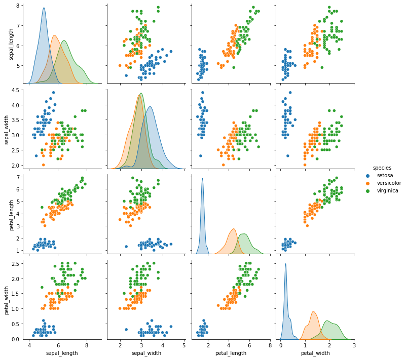
In order for classification to work, we’re looking to see that the groups of samples of different classes (here, species) do not overlap too much. We’re also looking at the shape of the groups of samples of each class.
Naive Bayes
Naive Bayes assumes that the features are uncorrelated (Naive) and that we can pick the most probable class. It can assume different distributions of the features conditioned on the class, though. We’ll use Gaussian Naive Bayes. Gaussian distributed samples in the plot above would be roughly ovals with more points at the center and uncorrelated Gaussian data would be distributed in circles, not ovals. We have some ovals and some overlap, but enough we can expect this classifier to work pretty well.
First we instantiate the classifier object with the constructor method.
gnb = GaussianNB()
We just made it exist so far, nothing more, so we can check its type.
type(gnb)
sklearn.naive_bayes.GaussianNB
We can also use the get_params method to see what it looks like.
gnb.get_params()
{'priors': None, 'var_smoothing': 1e-09}
Training a Model
Before we trian the model, we have to get our data out of the DataFrame, because our gnb.fit method takes arrays. We can use the values attribute
iris_df.values
array([[5.1, 3.5, 1.4, 0.2, 'setosa'],
       [4.9, 3.0, 1.4, 0.2, 'setosa'],
       [4.7, 3.2, 1.3, 0.2, 'setosa'],
       [4.6, 3.1, 1.5, 0.2, 'setosa'],
       [5.0, 3.6, 1.4, 0.2, 'setosa'],
       [5.4, 3.9, 1.7, 0.4, 'setosa'],
       [4.6, 3.4, 1.4, 0.3, 'setosa'],
       [5.0, 3.4, 1.5, 0.2, 'setosa'],
       [4.4, 2.9, 1.4, 0.2, 'setosa'],
       [4.9, 3.1, 1.5, 0.1, 'setosa'],
       [5.4, 3.7, 1.5, 0.2, 'setosa'],
       [4.8, 3.4, 1.6, 0.2, 'setosa'],
       [4.8, 3.0, 1.4, 0.1, 'setosa'],
       [4.3, 3.0, 1.1, 0.1, 'setosa'],
       [5.8, 4.0, 1.2, 0.2, 'setosa'],
       [5.7, 4.4, 1.5, 0.4, 'setosa'],
       [5.4, 3.9, 1.3, 0.4, 'setosa'],
       [5.1, 3.5, 1.4, 0.3, 'setosa'],
       [5.7, 3.8, 1.7, 0.3, 'setosa'],
       [5.1, 3.8, 1.5, 0.3, 'setosa'],
       [5.4, 3.4, 1.7, 0.2, 'setosa'],
       [5.1, 3.7, 1.5, 0.4, 'setosa'],
       [4.6, 3.6, 1.0, 0.2, 'setosa'],
       [5.1, 3.3, 1.7, 0.5, 'setosa'],
       [4.8, 3.4, 1.9, 0.2, 'setosa'],
       [5.0, 3.0, 1.6, 0.2, 'setosa'],
       [5.0, 3.4, 1.6, 0.4, 'setosa'],
       [5.2, 3.5, 1.5, 0.2, 'setosa'],
       [5.2, 3.4, 1.4, 0.2, 'setosa'],
       [4.7, 3.2, 1.6, 0.2, 'setosa'],
       [4.8, 3.1, 1.6, 0.2, 'setosa'],
       [5.4, 3.4, 1.5, 0.4, 'setosa'],
       [5.2, 4.1, 1.5, 0.1, 'setosa'],
       [5.5, 4.2, 1.4, 0.2, 'setosa'],
       [4.9, 3.1, 1.5, 0.2, 'setosa'],
       [5.0, 3.2, 1.2, 0.2, 'setosa'],
       [5.5, 3.5, 1.3, 0.2, 'setosa'],
       [4.9, 3.6, 1.4, 0.1, 'setosa'],
       [4.4, 3.0, 1.3, 0.2, 'setosa'],
       [5.1, 3.4, 1.5, 0.2, 'setosa'],
       [5.0, 3.5, 1.3, 0.3, 'setosa'],
       [4.5, 2.3, 1.3, 0.3, 'setosa'],
       [4.4, 3.2, 1.3, 0.2, 'setosa'],
       [5.0, 3.5, 1.6, 0.6, 'setosa'],
       [5.1, 3.8, 1.9, 0.4, 'setosa'],
       [4.8, 3.0, 1.4, 0.3, 'setosa'],
       [5.1, 3.8, 1.6, 0.2, 'setosa'],
       [4.6, 3.2, 1.4, 0.2, 'setosa'],
       [5.3, 3.7, 1.5, 0.2, 'setosa'],
       [5.0, 3.3, 1.4, 0.2, 'setosa'],
       [7.0, 3.2, 4.7, 1.4, 'versicolor'],
       [6.4, 3.2, 4.5, 1.5, 'versicolor'],
       [6.9, 3.1, 4.9, 1.5, 'versicolor'],
       [5.5, 2.3, 4.0, 1.3, 'versicolor'],
       [6.5, 2.8, 4.6, 1.5, 'versicolor'],
       [5.7, 2.8, 4.5, 1.3, 'versicolor'],
       [6.3, 3.3, 4.7, 1.6, 'versicolor'],
       [4.9, 2.4, 3.3, 1.0, 'versicolor'],
       [6.6, 2.9, 4.6, 1.3, 'versicolor'],
       [5.2, 2.7, 3.9, 1.4, 'versicolor'],
       [5.0, 2.0, 3.5, 1.0, 'versicolor'],
       [5.9, 3.0, 4.2, 1.5, 'versicolor'],
       [6.0, 2.2, 4.0, 1.0, 'versicolor'],
       [6.1, 2.9, 4.7, 1.4, 'versicolor'],
       [5.6, 2.9, 3.6, 1.3, 'versicolor'],
       [6.7, 3.1, 4.4, 1.4, 'versicolor'],
       [5.6, 3.0, 4.5, 1.5, 'versicolor'],
       [5.8, 2.7, 4.1, 1.0, 'versicolor'],
       [6.2, 2.2, 4.5, 1.5, 'versicolor'],
       [5.6, 2.5, 3.9, 1.1, 'versicolor'],
       [5.9, 3.2, 4.8, 1.8, 'versicolor'],
       [6.1, 2.8, 4.0, 1.3, 'versicolor'],
       [6.3, 2.5, 4.9, 1.5, 'versicolor'],
       [6.1, 2.8, 4.7, 1.2, 'versicolor'],
       [6.4, 2.9, 4.3, 1.3, 'versicolor'],
       [6.6, 3.0, 4.4, 1.4, 'versicolor'],
       [6.8, 2.8, 4.8, 1.4, 'versicolor'],
       [6.7, 3.0, 5.0, 1.7, 'versicolor'],
       [6.0, 2.9, 4.5, 1.5, 'versicolor'],
       [5.7, 2.6, 3.5, 1.0, 'versicolor'],
       [5.5, 2.4, 3.8, 1.1, 'versicolor'],
       [5.5, 2.4, 3.7, 1.0, 'versicolor'],
       [5.8, 2.7, 3.9, 1.2, 'versicolor'],
       [6.0, 2.7, 5.1, 1.6, 'versicolor'],
       [5.4, 3.0, 4.5, 1.5, 'versicolor'],
       [6.0, 3.4, 4.5, 1.6, 'versicolor'],
       [6.7, 3.1, 4.7, 1.5, 'versicolor'],
       [6.3, 2.3, 4.4, 1.3, 'versicolor'],
       [5.6, 3.0, 4.1, 1.3, 'versicolor'],
       [5.5, 2.5, 4.0, 1.3, 'versicolor'],
       [5.5, 2.6, 4.4, 1.2, 'versicolor'],
       [6.1, 3.0, 4.6, 1.4, 'versicolor'],
       [5.8, 2.6, 4.0, 1.2, 'versicolor'],
       [5.0, 2.3, 3.3, 1.0, 'versicolor'],
       [5.6, 2.7, 4.2, 1.3, 'versicolor'],
       [5.7, 3.0, 4.2, 1.2, 'versicolor'],
       [5.7, 2.9, 4.2, 1.3, 'versicolor'],
       [6.2, 2.9, 4.3, 1.3, 'versicolor'],
       [5.1, 2.5, 3.0, 1.1, 'versicolor'],
       [5.7, 2.8, 4.1, 1.3, 'versicolor'],
       [6.3, 3.3, 6.0, 2.5, 'virginica'],
       [5.8, 2.7, 5.1, 1.9, 'virginica'],
       [7.1, 3.0, 5.9, 2.1, 'virginica'],
       [6.3, 2.9, 5.6, 1.8, 'virginica'],
       [6.5, 3.0, 5.8, 2.2, 'virginica'],
       [7.6, 3.0, 6.6, 2.1, 'virginica'],
       [4.9, 2.5, 4.5, 1.7, 'virginica'],
       [7.3, 2.9, 6.3, 1.8, 'virginica'],
       [6.7, 2.5, 5.8, 1.8, 'virginica'],
       [7.2, 3.6, 6.1, 2.5, 'virginica'],
       [6.5, 3.2, 5.1, 2.0, 'virginica'],
       [6.4, 2.7, 5.3, 1.9, 'virginica'],
       [6.8, 3.0, 5.5, 2.1, 'virginica'],
       [5.7, 2.5, 5.0, 2.0, 'virginica'],
       [5.8, 2.8, 5.1, 2.4, 'virginica'],
       [6.4, 3.2, 5.3, 2.3, 'virginica'],
       [6.5, 3.0, 5.5, 1.8, 'virginica'],
       [7.7, 3.8, 6.7, 2.2, 'virginica'],
       [7.7, 2.6, 6.9, 2.3, 'virginica'],
       [6.0, 2.2, 5.0, 1.5, 'virginica'],
       [6.9, 3.2, 5.7, 2.3, 'virginica'],
       [5.6, 2.8, 4.9, 2.0, 'virginica'],
       [7.7, 2.8, 6.7, 2.0, 'virginica'],
       [6.3, 2.7, 4.9, 1.8, 'virginica'],
       [6.7, 3.3, 5.7, 2.1, 'virginica'],
       [7.2, 3.2, 6.0, 1.8, 'virginica'],
       [6.2, 2.8, 4.8, 1.8, 'virginica'],
       [6.1, 3.0, 4.9, 1.8, 'virginica'],
       [6.4, 2.8, 5.6, 2.1, 'virginica'],
       [7.2, 3.0, 5.8, 1.6, 'virginica'],
       [7.4, 2.8, 6.1, 1.9, 'virginica'],
       [7.9, 3.8, 6.4, 2.0, 'virginica'],
       [6.4, 2.8, 5.6, 2.2, 'virginica'],
       [6.3, 2.8, 5.1, 1.5, 'virginica'],
       [6.1, 2.6, 5.6, 1.4, 'virginica'],
       [7.7, 3.0, 6.1, 2.3, 'virginica'],
       [6.3, 3.4, 5.6, 2.4, 'virginica'],
       [6.4, 3.1, 5.5, 1.8, 'virginica'],
       [6.0, 3.0, 4.8, 1.8, 'virginica'],
       [6.9, 3.1, 5.4, 2.1, 'virginica'],
       [6.7, 3.1, 5.6, 2.4, 'virginica'],
       [6.9, 3.1, 5.1, 2.3, 'virginica'],
       [5.8, 2.7, 5.1, 1.9, 'virginica'],
       [6.8, 3.2, 5.9, 2.3, 'virginica'],
       [6.7, 3.3, 5.7, 2.5, 'virginica'],
       [6.7, 3.0, 5.2, 2.3, 'virginica'],
       [6.3, 2.5, 5.0, 1.9, 'virginica'],
       [6.5, 3.0, 5.2, 2.0, 'virginica'],
       [6.2, 3.4, 5.4, 2.3, 'virginica'],
       [5.9, 3.0, 5.1, 1.8, 'virginica']], dtype=object)
Then we create test an train splits of our data. we’ll to equal parts (test_size = .5) and set the random state so that we call get the same result
X_train, X_test,  y_train, y_test = train_test_split(iris_df.values[:,:4],
                                                     iris_df.values[:,-1],
                                                    test_size = .5,
                                                    random_state =0)
try it yourself!
rerun the test
train_test_splitwithout random state, to see how it’s differentchange the
test_sizeto different sizes and see what happens.
Now we use the training data to fit our model.
gnb.fit(X_train, y_train)
GaussianNB()
Now we can predict using the test data’s features only.
y_pred = gnb.predict(X_test)
y_pred
array(['virginica', 'versicolor', 'setosa', 'virginica', 'setosa',
       'virginica', 'setosa', 'versicolor', 'versicolor', 'versicolor',
       'versicolor', 'versicolor', 'versicolor', 'versicolor',
       'versicolor', 'setosa', 'versicolor', 'versicolor', 'setosa',
       'setosa', 'virginica', 'versicolor', 'setosa', 'setosa',
       'virginica', 'setosa', 'setosa', 'versicolor', 'versicolor',
       'setosa', 'virginica', 'versicolor', 'setosa', 'virginica',
       'virginica', 'versicolor', 'setosa', 'versicolor', 'versicolor',
       'versicolor', 'virginica', 'setosa', 'virginica', 'setosa',
       'setosa', 'versicolor', 'virginica', 'virginica', 'versicolor',
       'virginica', 'versicolor', 'virginica', 'versicolor', 'versicolor',
       'virginica', 'versicolor', 'versicolor', 'virginica', 'versicolor',
       'virginica', 'versicolor', 'setosa', 'virginica', 'versicolor',
       'versicolor', 'versicolor', 'versicolor', 'virginica', 'setosa',
       'setosa', 'virginica', 'versicolor', 'setosa', 'setosa',
       'versicolor'], dtype='<U10')
We can compare this to the y_test to see how well our classifier works.
y_test
array(['virginica', 'versicolor', 'setosa', 'virginica', 'setosa',
       'virginica', 'setosa', 'versicolor', 'versicolor', 'versicolor',
       'virginica', 'versicolor', 'versicolor', 'versicolor',
       'versicolor', 'setosa', 'versicolor', 'versicolor', 'setosa',
       'setosa', 'virginica', 'versicolor', 'setosa', 'setosa',
       'virginica', 'setosa', 'setosa', 'versicolor', 'versicolor',
       'setosa', 'virginica', 'versicolor', 'setosa', 'virginica',
       'virginica', 'versicolor', 'setosa', 'versicolor', 'versicolor',
       'versicolor', 'virginica', 'setosa', 'virginica', 'setosa',
       'setosa', 'versicolor', 'virginica', 'virginica', 'virginica',
       'virginica', 'versicolor', 'virginica', 'versicolor', 'versicolor',
       'virginica', 'virginica', 'virginica', 'virginica', 'versicolor',
       'virginica', 'versicolor', 'setosa', 'virginica', 'versicolor',
       'versicolor', 'versicolor', 'versicolor', 'virginica', 'setosa',
       'setosa', 'virginica', 'versicolor', 'setosa', 'setosa',
       'versicolor'], dtype=object)
We can simply use base python to get the number correct with a boolean and sum since False turns to 0 and True to 1.
sum(y_pred == y_test)
71
and compare that with the total
len(y_pred)
75
or compute accuracy
sum(y_pred == y_test)/len(y_pred)
0.9466666666666667
Questions after class
I’m curious about other classifiers
Great! We’ll see more Friday, next week, and next month. You’re also encouraged to try out others and experiment with sci-kit learn.
How we got the values from the DataFrame
A DataFrame is an object and one of the attributes is values, we accessed that directly. However, there is a new, safer way through the to_numpy method.