Class 22: More Regression, More Evaluation and LASSO
log prismia chat
say hello in the zoom chat
import matplotlib.pyplot as plt
import seaborn as sns
import numpy as np
import pandas as pd
from sklearn import datasets, linear_model
from sklearn.metrics import mean_squared_error, r2_score
from sklearn.model_selection import cross_val_score
from sklearn.model_selection import train_test_split

# Load the diabetes dataset
diabetes_X, diabetes_y = datasets.load_diabetes(return_X_y=True)
Questions after class Monday
Some good questions were asked on the form Monday. Check the notes for insight on the r2_score and mean_square_error.
Review of Test Train splits
X_train,X_test, y_train,y_test = train_test_split(diabetes_X, diabetes_y ,
                                                  test_size=20,random_state=0)
What metric does the score method of LinearRegression use?
regr = linear_model.LinearRegression()
regr.fit(X_train, y_train)
LinearRegression()
regr.score(X_test,y_test)
0.5195208400616668
y_pred = regr.predict(X_test)
r2_score(y_test,y_pred)
0.5195208400616668
mean_squared_error(y_test,y_pred)
2850.3176917525775
Digging in deeper to the Linear Regression model
Linear regression fitting involvles learning the coefficients
regr.coef_
array([ -32.3074285 , -257.44432972,  513.31945939,  338.46656647,
       -766.86983748,  455.85416891,   92.55795582,  184.75163454,
        734.92318647,   82.7231425 ])
and an intercept
regr.intercept_
152.39189054201842
The linear regression model is
wehere it stores \(w\) in the coef_ attribute and b as the intercept_
We can check how this works by multiplying one sample by the coefficients, to get a vector
X_test[0]*regr.coef_
array([ -0.64334474, -13.0473092 ,  53.80033982,  23.71721361,
        27.58260658, -12.16168908,  -2.31326921,  -0.47892464,
         2.72784249,   3.33733048])
then taking the sum and adding the intercept
np.sum(X_test[0]*regr.coef_) + regr.intercept_
234.9126866563482
and then comparing to the predictions.
y_pred[0]
234.91268665634823
These are not exactly the same due to float rounding erros, but they’re very close.
We can also check for the whole test set
errors = np.sum(X_test*regr.coef_,axis=1) + regr.intercept_ -y_pred
errors
array([-2.84217094e-14,  0.00000000e+00,  0.00000000e+00,  0.00000000e+00,
        0.00000000e+00,  0.00000000e+00,  0.00000000e+00,  0.00000000e+00,
        0.00000000e+00,  0.00000000e+00,  0.00000000e+00,  0.00000000e+00,
        1.42108547e-14,  0.00000000e+00,  0.00000000e+00,  0.00000000e+00,
        0.00000000e+00, -1.42108547e-14, -2.84217094e-14,  0.00000000e+00])
and confirm these are very small
np.max(errors)
1.4210854715202004e-14
It’s doing linear regression as we expected.
Changing the complexity in Linear regression
It can be important to also know what the model is really doing and see how different features are used or not. Maybe, for example all of the features are expensive to measure, but for testing we measured a lot of them. We might want to simultaneously learn which features we actually need and the linear model.
LASSO can do that for us it’s objective is like linear regression, but it adds an extra term. This term forces some of the learned coefficients to be 0. Mulitplying by 0 gives 0, so that’s like throwing away that feature. The term is called the \(1-norm\), the details of the math are not important here, just the idea that it can reduce the number of features used as well.
lasso = linear_model.Lasso()
lasso.fit(X_train, y_train)
lasso.score(X_test,y_test)
0.4224899448032938
It uses many fewer
lasso.coef_
array([  0.        ,  -0.        , 358.27498703,   9.7141813 ,
         0.        ,   0.        ,  -0.        ,   0.        ,
       309.50796119,   0.        ])
It has a parameter alpha that must be >0 that we can use to control how many features it uses. When alpha = 0 it’s the same as linear regression, but the regular linear regression estimator uses a more numerically stable algorithm for the fit method
lasso2 = linear_model.Lasso(alpha=.5)
lasso2.fit(X_train, y_train)
lasso2.score(X_test,y_test)
0.5272242529276977
We see tha fewer are 0 now.
lasso2.coef_
array([  0.        ,  -0.        , 466.09039819, 140.20195776,
        -0.        ,  -0.        , -61.96474668,   0.        ,
       405.95829094,   0.        ])
regr.score(X_train, y_train)
0.5170933599105026
lasso2.score(X_train, y_train)
0.4516267981295532
lasso_cv = cross_val_score(lasso2, diabetes_X, diabetes_y)
lasso_cv
array([0.3712605 , 0.45675648, 0.45066569, 0.42134051, 0.47736463])
regr_cv = cross_val_score(regr,diabetes_X, diabetes_y )
regr_cv
array([0.42955643, 0.52259828, 0.4826784 , 0.42650827, 0.55024923])
np.mean(lasso_cv), np.mean(regr_cv)
(0.43547756049731523, 0.48231812211149394)
cross_val_score(regr,diabetes_X, diabetes_y ,cv=10)
array([0.55614411, 0.23056092, 0.35357777, 0.62190498, 0.26587602,
       0.61819338, 0.41815916, 0.43515232, 0.43436983, 0.68568514])
We can do cross validation for all three of these models and look at both the mean and the standard deviation. The mean tells us how well on average each model does on different subsets of the data.
The standard deviation is a measure of spread of the scores. For intuition, another measure of spread is max(cv_scores) - min(cv_scores).
regr_cv = cross_val_score(regr,diabetes_X, diabetes_y ,cv=10)
np.mean(regr_cv), np.std(regr_cv)
(0.461962361958337, 0.14698789185375888)
lasso_cv = cross_val_score(lasso,diabetes_X, diabetes_y ,cv=10)
np.mean(lasso_cv), np.std(lasso_cv)
(0.3211351084864853, 0.09122225780232662)
lasso2_cv = cross_val_score(lasso2,diabetes_X, diabetes_y ,cv=10)
np.mean(lasso2_cv), np.std(lasso2_cv)
(0.41808972445133297, 0.11927596370400496)
Questions after class
What does the cv parameter in cross_val_score do?
First, let’s look at the help.
help(cross_val_score)
Help on function cross_val_score in module sklearn.model_selection._validation:

cross_val_score(estimator, X, y=None, *, groups=None, scoring=None, cv=None, n_jobs=None, verbose=0, fit_params=None, pre_dispatch='2*n_jobs', error_score=nan)
    Evaluate a score by cross-validation

    Read more in the :ref:`User Guide <cross_validation>`.

    Parameters
    ----------
    estimator : estimator object implementing 'fit'
        The object to use to fit the data.

    X : array-like of shape (n_samples, n_features)
        The data to fit. Can be for example a list, or an array.

    y : array-like of shape (n_samples,) or (n_samples, n_outputs),             default=None
        The target variable to try to predict in the case of
        supervised learning.

    groups : array-like of shape (n_samples,), default=None
        Group labels for the samples used while splitting the dataset into
        train/test set. Only used in conjunction with a "Group" :term:`cv`
        instance (e.g., :class:`GroupKFold`).

    scoring : str or callable, default=None
        A str (see model evaluation documentation) or
        a scorer callable object / function with signature
        ``scorer(estimator, X, y)`` which should return only
        a single value.

        Similar to :func:`cross_validate`
        but only a single metric is permitted.

        If None, the estimator's default scorer (if available) is used.

    cv : int, cross-validation generator or an iterable, default=None
        Determines the cross-validation splitting strategy.
        Possible inputs for cv are:

        - None, to use the default 5-fold cross validation,
        - int, to specify the number of folds in a `(Stratified)KFold`,
        - :term:`CV splitter`,
        - An iterable yielding (train, test) splits as arrays of indices.

        For int/None inputs, if the estimator is a classifier and ``y`` is
        either binary or multiclass, :class:`StratifiedKFold` is used. In all
        other cases, :class:`KFold` is used. These splitters are instantiated
        with `shuffle=False` so the splits will be the same across calls.

        Refer :ref:`User Guide <cross_validation>` for the various
        cross-validation strategies that can be used here.

        .. versionchanged:: 0.22
            ``cv`` default value if None changed from 3-fold to 5-fold.

    n_jobs : int, default=None
        Number of jobs to run in parallel. Training the estimator and computing
        the score are parallelized over the cross-validation splits.
        ``None`` means 1 unless in a :obj:`joblib.parallel_backend` context.
        ``-1`` means using all processors. See :term:`Glossary <n_jobs>`
        for more details.

    verbose : int, default=0
        The verbosity level.

    fit_params : dict, default=None
        Parameters to pass to the fit method of the estimator.

    pre_dispatch : int or str, default='2*n_jobs'
        Controls the number of jobs that get dispatched during parallel
        execution. Reducing this number can be useful to avoid an
        explosion of memory consumption when more jobs get dispatched
        than CPUs can process. This parameter can be:

            - None, in which case all the jobs are immediately
              created and spawned. Use this for lightweight and
              fast-running jobs, to avoid delays due to on-demand
              spawning of the jobs

            - An int, giving the exact number of total jobs that are
              spawned

            - A str, giving an expression as a function of n_jobs,
              as in '2*n_jobs'

    error_score : 'raise' or numeric, default=np.nan
        Value to assign to the score if an error occurs in estimator fitting.
        If set to 'raise', the error is raised.
        If a numeric value is given, FitFailedWarning is raised.

        .. versionadded:: 0.20

    Returns
    -------
    scores : ndarray of float of shape=(len(list(cv)),)
        Array of scores of the estimator for each run of the cross validation.

    Examples
    --------
    >>> from sklearn import datasets, linear_model
    >>> from sklearn.model_selection import cross_val_score
    >>> diabetes = datasets.load_diabetes()
    >>> X = diabetes.data[:150]
    >>> y = diabetes.target[:150]
    >>> lasso = linear_model.Lasso()
    >>> print(cross_val_score(lasso, X, y, cv=3))
    [0.33150734 0.08022311 0.03531764]

    See Also
    ---------
    cross_validate : To run cross-validation on multiple metrics and also to
        return train scores, fit times and score times.

    cross_val_predict : Get predictions from each split of cross-validation for
        diagnostic purposes.

    sklearn.metrics.make_scorer : Make a scorer from a performance metric or
        loss function.
It does different things, depending on what type of value we pass it. We passed it an int (10), so what it did was split the data into 10 groups and then trains on 9/10 of those parts and tests on the last one. Then it iterates over those folds.
For classification, it can take into consideration the target value (classes) and an additionally specified group in the data. A good visualization of what it does is shown in the sklearn docs.
It uses StratifiedKfold for classification, but since we’re using regression it will use KFold. test_train_split uses ShuffleSplit by default, let’s load that too to see what it does.
Warning
The key in the following is to get the concepts not all of the details in how I evaluate and visualize. I could have made figures separately to explain the concept, but I like to show that Python is self contained.
from sklearn.model_selection import KFold, ShuffleSplit
kf = KFold(n_splits = 10)
When we use the split method it gives us a generator.
kf.split(diabetes_X, diabetes_y)
<generator object _BaseKFold.split at 0x7fd98e8c5550>
We can use this in a loop to get the list of indices that will be used to get the test and train data for each fold. To visualize what this is doing, see below.
N_samples = len(diabetes_y)
kf_tt_df = pd.DataFrame(index=list(range(N_samples)))
i = 1
for train_idx, test_idx in kf.split(diabetes_X, diabetes_y):
    kf_tt_df['split ' + str(i)] = ['unused']*N_samples
    kf_tt_df['split ' + str(i)][train_idx] = 'Train'
    kf_tt_df['split ' + str(i)][test_idx] = 'Test'
    i +=1
We can count how many times ‘Test’ and ‘Train’ appear
count_test = lambda part: len([v for v in part if v=='Test'])
count_train = lambda part: len([v for v in part if v=='Train'])
When we apply this along axis=1 we to check that each sample is used in exactly 1 test set how may times each sample is used
sum(kf_tt_df.apply(count_test,axis = 1) ==1)
442
and exactly 9 training sets
sum(kf_tt_df.apply(count_test,axis = 1) ==9)
0
the describe helps ensure that all fo the values are exa
We can also visualize:
cmap = sns.color_palette("tab10",10)
g = sns.heatmap(kf_tt_df.replace({'Test':1,'Train':0}),cmap=cmap[7:9],cbar_kws={'ticks':[.25,.75]},linewidths=0,
    linecolor='gray')
colorbar = g.collections[0].colorbar
colorbar.set_ticklabels(['Train','Test'])
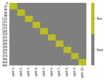
Note that unlike test_train_split this does not always randomize and shuffle the data before splitting.
If we apply those lambda functions along axis=0, we can see the size of each test set
kf_tt_df.apply(count_test,axis = 0)
split 1     45
split 2     45
split 3     44
split 4     44
split 5     44
split 6     44
split 7     44
split 8     44
split 9     44
split 10    44
dtype: int64
and training set:
kf_tt_df.apply(count_train,axis = 0)
split 1     397
split 2     397
split 3     398
split 4     398
split 5     398
split 6     398
split 7     398
split 8     398
split 9     398
split 10    398
dtype: int64
We can verify that these splits are the same size as what test_train_split does using the right settings. 10-fold splits the data into 10 parts and tests on 1, so that makes a test size of 1/10=.1, so we can use the train_test_split and check the length.
X_train2,X_test2, y_train2,y_test2 = train_test_split(diabetes_X, diabetes_y ,
                                                  test_size=.1,random_state=0)

[len(split) for split in [X_train2,X_test2,]]
Under the hood train_test_split uses ShuffleSplit
We can do a similar experiment as above to see what ShuffleSplit does.
skf = ShuffleSplit(10)
N_samples = len(diabetes_y)
ss_tt_df = pd.DataFrame(index=list(range(N_samples)))
i = 1
for train_idx, test_idx in skf.split(diabetes_X, diabetes_y):
    ss_tt_df['split ' + str(i)] = ['unused']*N_samples
    ss_tt_df['split ' + str(i)][train_idx] = 'Train'
    ss_tt_df['split ' + str(i)][test_idx] = 'Test'
    i +=1

ss_tt_df
| split 1 | split 2 | split 3 | split 4 | split 5 | split 6 | split 7 | split 8 | split 9 | split 10 | |
|---|---|---|---|---|---|---|---|---|---|---|
| 0 | Train | Train | Train | Train | Train | Train | Train | Train | Train | Train |
| 1 | Train | Train | Train | Test | Train | Train | Train | Train | Train | Train |
| 2 | Train | Train | Train | Train | Train | Train | Train | Train | Train | Train |
| 3 | Train | Train | Train | Train | Train | Train | Train | Train | Train | Train |
| 4 | Train | Train | Train | Train | Train | Train | Train | Train | Train | Train |
| ... | ... | ... | ... | ... | ... | ... | ... | ... | ... | ... |
| 437 | Train | Train | Train | Train | Test | Train | Train | Train | Test | Train |
| 438 | Test | Train | Train | Train | Train | Train | Train | Train | Train | Train |
| 439 | Train | Train | Train | Train | Train | Train | Train | Train | Train | Train |
| 440 | Train | Train | Train | Train | Train | Train | Train | Train | Train | Train |
| 441 | Train | Train | Train | Train | Test | Train | Train | Train | Train | Test |
442 rows × 10 columns
And plot
cmap = sns.color_palette("tab10",10)
g = sns.heatmap(ss_tt_df.replace({'Test':1,'Train':0}),cmap=cmap[7:9],cbar_kws={'ticks':[.25,.75]},linewidths=0,
    linecolor='gray')
colorbar = g.collections[0].colorbar
colorbar.set_ticklabels(['Train','Test'])
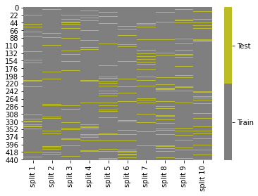
Now, we see the samples in each training set (gray along the columns) are a random subset of all of all of the samples.
And check the usage of each sample
sum(ss_tt_df.apply(count_test,axis = 1) ==1)
172
and exactly 9 training sets
sum(ss_tt_df.apply(count_test,axis = 1) ==9)
0
And the size of the splits
ss_tt_df.apply(count_test,axis = 0)
split 1     45
split 2     45
split 3     45
split 4     45
split 5     45
split 6     45
split 7     45
split 8     45
split 9     45
split 10    45
dtype: int64
and training set:
ss_tt_df.apply(count_train,axis = 0)
split 1     397
split 2     397
split 3     397
split 4     397
split 5     397
split 6     397
split 7     397
split 8     397
split 9     397
split 10    397
dtype: int64
Again the same sizes