33. Predicting with Neural Networks#

from scipy.special import expit
from sklearn.datasets import make_classification
from sklearn.neural_network import MLPClassifier

from sklearn import svm
import pandas as pd
import numpy as np
import sklearn

from sklearn import datasets
import matplotlib.pyplot as plt
from sklearn import model_selection
# from skearn.model_selection import train_test_split

import seaborn as sns
sns.set_theme(palette='colorblind')

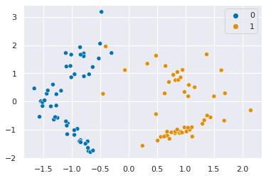
Today, were going to use very simple data in order to examin how a neural network works.

X, y = make_classification(n_samples=100, random_state=1,n_features=2,n_redundant=0)
X_train, X_test, y_train, y_test = model_selection.train_test_split(X, y, stratify=y,
                          random_state=1)
sns.scatterplot(x=X[:,0],y=X[:,1],hue=y)
<AxesSubplot:>
../_images/2021-12-03_3_1.png

First, we’ll train and score a tiny neural net: with 1 hidden layer of 1 neuron.

clf = MLPClassifier(
  hidden_layer_sizes=(1), # 1 hidden layer, 1 aritficial neuron
  max_iter=100, # maximum 100 interations in optimization
  alpha=1e-4, # regularization
  solver="lbfgs", #optimization algorithm  
  verbose=10, # how much detail to print
  activation= 'identity' # how to transform the hidden layer beofore passing it to the next layer
)
clf.fit(X_train, y_train)

clf.score(X_test, y_test)
RUNNING THE L-BFGS-B CODE

           * * *

Machine precision = 2.220D-16
 N =            5     M =           10

At X0         0 variables are exactly at the bounds

At iterate    0    f=  2.34381D+00    |proj g|=  1.10750D+00

At iterate    1    f=  1.15884D+00    |proj g|=  5.22275D-01

At iterate    2    f=  7.01374D-01    |proj g|=  9.09004D-02

At iterate    3    f=  6.76700D-01    |proj g|=  9.43005D-02

At iterate    4    f=  1.73953D-01    |proj g|=  3.30244D-01

At iterate    5    f=  5.13513D-02    |proj g|=  2.94368D-02

At iterate    6    f=  4.99313D-02    |proj g|=  1.89818D-02

At iterate    7    f=  4.87264D-02    |proj g|=  5.76625D-03

At iterate    8    f=  4.86119D-02    |proj g|=  4.00697D-03

At iterate    9    f=  4.84878D-02    |proj g|=  1.92688D-03

At iterate   10    f=  4.83939D-02    |proj g|=  1.64081D-03

At iterate   11    f=  4.82015D-02    |proj g|=  3.84407D-03

At iterate   12    f=  4.80076D-02    |proj g|=  3.82976D-03

At iterate   13    f=  4.79248D-02    |proj g|=  9.15466D-04

At iterate   14    f=  4.79198D-02    |proj g|=  2.37753D-04

At iterate   15    f=  4.79196D-02    |proj g|=  5.87358D-05

           * * *

Tit   = total number of iterations
Tnf   = total number of function evaluations
Tnint = total number of segments explored during Cauchy searches
Skip  = number of BFGS updates skipped
Nact  = number of active bounds at final generalized Cauchy point
Projg = norm of the final projected gradient
F     = final function value

           * * *

   N    Tit     Tnf  Tnint  Skip  Nact     Projg        F
    5     15     18      1     0     0   5.874D-05   4.792D-02
  F =   4.7919620535136993E-002

CONVERGENCE: NORM_OF_PROJECTED_GRADIENT_<=_PGTOL            
 This problem is unconstrained.
1.0

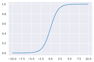
Now we can see that it actually has another activation, that we didn’t change the output layer still has a logistic activation layer, which we want. If we didn’t then the output layer wouldn’t be able to be interpretted as a probability, because probability always needs to be between 0 and 1.

clf.out_activation_
'logistic'

The logistic function looks like this:

x_logistic = np.linspace(-10,10,100)
y_logistic = expit(x_logistic)
plt.plot(x_logistic,y_logistic)
[<matplotlib.lines.Line2D at 0x7f49d5ab9760>]
../_images/2021-12-03_9_1.png

The fit method learned the following weights:

clf.coefs_
[array([[-6.85186628],
        [ 0.19720034]]),
 array([[-1.91807161]])]

and biases

clf.intercepts_
[array([0.02652099]), array([5.74570119])]

These are called coefficients and intercepts because the weights are mutliplied by the inputs and the biases you can interpret as geometrically as shifting things, like a line intercept (recall y=mx+b)

33.1. Reconstructing the Predict method#

we’ll use an acutally new point, we can make one up

type([[-1,2]])
list

we want a numpy array so we will cast it

pt = np.array([[-1,2]])
type(pt)
numpy.ndarray

numpy’s matmul does matrix multiplicaion (multiply columns by rows element wise and sum)

\[f(x) = W_2g(W_1^T x +b_1) + b_2 \]

the \(g\) is the activation function, which we set to identity \(g(x) = x\) so we don’t have to do more

np.matmul(pt,clf.coefs_[0]) + clf.intercepts_[0])*clf.coefs_[1] + clf.intercepts_[1])
  Input In [11]
    np.matmul(pt,clf.coefs_[0]) + clf.intercepts_[0])*clf.coefs_[1] + clf.intercepts_[1])
                                                    ^
SyntaxError: unmatched ')'

but we’re not quite done, the output layer still transforms using the logistic function, which is also known as expit and we have imported from scipy.

expit((np.matmul(pt,clf.coefs_[0]) + clf.intercepts_[0])*clf.coefs_[1] + clf.intercepts_[1])
array([[0.00027347]])

We can compare this to the classifier’s output. It outputs a probability for each class, we only comptued the probabilyt of the 1 class.

clf.predict_proba(pt)
array([[9.99726525e-01, 2.73474984e-04]])

and we can see how it predicts on that point.

clf.predict(pt)
array([0])

A single artificial neuron like the function below. where it has parameters that have to be determined before we can use it on an input vector.

def aritificial_neuron_template(activation,weights,bias,inputs):
    '''
    simple artificial neuron

    Parameters
    ----------
    activation : function
        activation function of the neuron
    weights : numpy aray
        wights for summing inputs
    bias: numpy array
        bias term added to the weighted sum
    inputs : numpy array
        input to the neuron

    '''
    return activation(np.matmul(inputs,weights) +bias)

# two common activation functions
identity_activation = lambda x: x
logistic_activation = lambda x: expit(x)

When we instantiate the multilyer perceptron object, MLPClassifier, we pick the activation function and when we give data to the fit method, we get the weights and biases.

A neural network passes the data to the hidden layer, and the output of the hidden layer to the output layer. In our neural network, we have just one neuron at each layer.

So the predict_proba method is the same as the following:

aritificial_neuron_template(logistic_activation,clf.coefs_[1],clf.intercepts_[1],
                 aritificial_neuron_template(identity_activation,clf.coefs_[0],
                   clf.intercepts_[0],pt))
array([[0.00027347]])

To make this easier to read, we can make the intermediate neurons their own lambda functions.

hidden_neuron = lambda x: aritificial_neuron_template(identity_activation,clf.coefs_[0],clf.intercepts_[0],x)
output_neuron = lambda x: aritificial_neuron_template(expit,clf.coefs_[1],clf.intercepts_[1],x)

output_neuron(hidden_neuron(pt))
array([[0.00027347]])

We can confirm that this works the same as the predict probability method:

clf.predict_proba(pt)
array([[9.99726525e-01, 2.73474984e-04]])

33.2. More Features and More Hidden Neurons#

First, we’ll sample more features and then train a new classifier

X, y = make_classification(n_samples=100, random_state=1,n_features=4,n_redundant=0)
X_train, X_test, y_train, y_test = train_test_split(X, y, stratify=y,
                                                    random_state=5)
pt_4d =np.asarray([[-1,-2,2,-1],[1.5,0,.5,1]])
clf_4d = MLPClassifier(
    hidden_layer_sizes=(1),
    max_iter=5000,
    alpha=1e-4,
    solver="lbfgs",
    verbose=10,
    activation= 'identity'
)

clf_4d.fit(X_train, y_train)


clf_4d.score(X_test, y_test)
---------------------------------------------------------------------------
NameError                                 Traceback (most recent call last)
Input In [19], in <cell line: 2>()
      1 X, y = make_classification(n_samples=100, random_state=1,n_features=4,n_redundant=0)
----> 2 X_train, X_test, y_train, y_test = train_test_split(X, y, stratify=y,
      3                                                     random_state=5)
      4 pt_4d =np.asarray([[-1,-2,2,-1],[1.5,0,.5,1]])
      5 clf_4d = MLPClassifier(
      6     hidden_layer_sizes=(1),
      7     max_iter=5000,
   (...)
     11     activation= 'identity'
     12 )

NameError: name 'train_test_split' is not defined

We can look at this data

df = pd.DataFrame(X,columns=['x0','x1','x2','x3'])
df['y'] = y
sns.pairplot(df,hue='y')
<seaborn.axisgrid.PairGrid at 0x7f49d554acd0>
../_images/2021-12-03_38_1.png

and based on this, we’ll pick a new pair of points to test on:

pt_4d =np.asarray([[-2,2,2,-2],[1.5,0,-1,3]])

This neural network is just like the one before:

hidden_neuron_4d = lambda x: aritificial_neuron_template(identity_activation,
                                                         clf_4d.coefs_[0],clf_4d.intercepts_[0],x)
output_neuron_4d = lambda x: aritificial_neuron_template(logistic_activation,
                                                         clf_4d.coefs_[1],clf_4d.intercepts_[1],x)


output_neuron_4d(hidden_neuron_4d(pt_4d))
---------------------------------------------------------------------------
NameError                                 Traceback (most recent call last)
Input In [22], in <cell line: 7>()
      1 hidden_neuron_4d = lambda x: aritificial_neuron_template(identity_activation,
      2                                                          clf_4d.coefs_[0],clf_4d.intercepts_[0],x)
      3 output_neuron_4d = lambda x: aritificial_neuron_template(logistic_activation,
      4                                                          clf_4d.coefs_[1],clf_4d.intercepts_[1],x)
----> 7 output_neuron_4d(hidden_neuron_4d(pt_4d))

Input In [22], in <lambda>(x)
      1 hidden_neuron_4d = lambda x: aritificial_neuron_template(identity_activation,
----> 2                                                          clf_4d.coefs_[0],clf_4d.intercepts_[0],x)
      3 output_neuron_4d = lambda x: aritificial_neuron_template(logistic_activation,
      4                                                          clf_4d.coefs_[1],clf_4d.intercepts_[1],x)
      7 output_neuron_4d(hidden_neuron_4d(pt_4d))

NameError: name 'clf_4d' is not defined
clf_4d.predict_proba(pt_4d)
---------------------------------------------------------------------------
NameError                                 Traceback (most recent call last)
Input In [23], in <cell line: 1>()
----> 1 clf_4d.predict_proba(pt_4d)

NameError: name 'clf_4d' is not defined

However, remember this one was not as accurate:

clf_4d.score(X_test, y_test)
---------------------------------------------------------------------------
NameError                                 Traceback (most recent call last)
Input In [24], in <cell line: 1>()
----> 1 clf_4d.score(X_test, y_test)

NameError: name 'clf_4d' is not defined

To try imporving it, we will add more layers and a different activation function:

clf_4d_4h = MLPClassifier(
    hidden_layer_sizes=(4),
    max_iter=500,
    alpha=1e-4,
    solver="lbfgs",
    verbose=10,
    activation='logistic'
)

clf_4d_4h.fit(X_train, y_train)


clf_4d_4h.score(X_test, y_test)
RUNNING THE L-BFGS-B CODE

           * * *

Machine precision = 2.220D-16
 N =           17     M =           10

At X0         0 variables are exactly at the bounds

At iterate    0    f=  7.39798D-01    |proj g|=  7.60692D-02

At iterate    1    f=  7.26134D-01    |proj g|=  1.50172D-01

At iterate    2    f=  6.76306D-01    |proj g|=  5.00387D-02

At iterate    3    f=  6.49665D-01    |proj g|=  5.44130D-02

At iterate    4    f=  5.25451D-01    |proj g|=  2.15246D-01

At iterate    5    f=  4.23006D-01    |proj g|=  2.05051D-01

At iterate    6    f=  1.40544D-01    |proj g|=  4.57748D-02

At iterate    7    f=  1.28650D-01    |proj g|=  3.78602D-02

At iterate    8    f=  9.53885D-02    |proj g|=  1.72836D-02

At iterate    9    f=  8.44214D-02    |proj g|=  1.09155D-02

At iterate   10    f=  7.04328D-02    |proj g|=  9.14381D-03

At iterate   11    f=  6.48659D-02    |proj g|=  4.82831D-03

At iterate   12    f=  5.98470D-02    |proj g|=  8.90528D-03

At iterate   13    f=  5.28991D-02    |proj g|=  1.53860D-02

At iterate   14    f=  4.39896D-02    |proj g|=  4.77902D-03

At iterate   15    f=  4.25224D-02    |proj g|=  4.69741D-03

At iterate   16    f=  4.07994D-02    |proj g|=  2.21123D-03

At iterate   17    f=  3.95558D-02    |proj g|=  5.16637D-03

At iterate   18    f=  3.66907D-02    |proj g|=  1.92226D-03

At iterate   19    f=  3.48200D-02    |proj g|=  4.93243D-03

At iterate   20    f=  3.41086D-02    |proj g|=  3.44697D-03

At iterate   21    f=  3.36224D-02    |proj g|=  3.44515D-03

At iterate   22    f=  3.20026D-02    |proj g|=  1.72674D-03

At iterate   23    f=  3.14277D-02    |proj g|=  1.42370D-03

At iterate   24    f=  3.10135D-02    |proj g|=  6.81954D-04

At iterate   25    f=  3.09077D-02    |proj g|=  1.83127D-04

At iterate   26    f=  3.08484D-02    |proj g|=  3.98862D-04

At iterate   27    f=  3.07962D-02    |proj g|=  5.98374D-04

At iterate   28    f=  3.06875D-02    |proj g|=  7.19001D-04

At iterate   29    f=  3.06252D-02    |proj g|=  5.18501D-04

At iterate   30    f=  3.03507D-02    |proj g|=  9.92446D-04

At iterate   31    f=  2.94907D-02    |proj g|=  2.96420D-03

At iterate   32    f=  2.94497D-02    |proj g|=  2.94538D-03

At iterate   33    f=  2.93113D-02    |proj g|=  3.38284D-03

At iterate   34    f=  2.91957D-02    |proj g|=  2.96397D-03

At iterate   35    f=  2.90365D-02    |proj g|=  1.76136D-03

At iterate   36    f=  2.87991D-02    |proj g|=  2.46091D-04

At iterate   37    f=  2.87555D-02    |proj g|=  2.75138D-04

At iterate   38    f=  2.86773D-02    |proj g|=  4.07157D-04

At iterate   39    f=  2.84211D-02    |proj g|=  1.24944D-03

At iterate   40    f=  2.70889D-02    |proj g|=  2.96296D-03

At iterate   41    f=  2.67305D-02    |proj g|=  5.63750D-03

At iterate   42    f=  2.48073D-02    |proj g|=  2.81205D-03

At iterate   43    f=  2.35024D-02    |proj g|=  1.05261D-03

At iterate   44    f=  2.30253D-02    |proj g|=  6.67917D-04

At iterate   45    f=  2.29028D-02    |proj g|=  5.38500D-04

At iterate   46    f=  2.27677D-02    |proj g|=  8.60951D-04

At iterate   47    f=  2.25993D-02    |proj g|=  2.58897D-04

At iterate   48    f=  2.25169D-02    |proj g|=  2.80334D-04

At iterate   49    f=  2.23866D-02    |proj g|=  3.90709D-04

At iterate   50    f=  2.22414D-02    |proj g|=  3.80260D-04

At iterate   51    f=  2.18184D-02    |proj g|=  1.91141D-04

At iterate   52    f=  2.17625D-02    |proj g|=  2.42250D-04
 This problem is unconstrained.
1.0
At iterate   53    f=  2.16786D-02    |proj g|=  2.92993D-04

At iterate   54    f=  2.15285D-02    |proj g|=  2.69982D-04

At iterate   55    f=  2.15015D-02    |proj g|=  5.21127D-04

At iterate   56    f=  2.12361D-02    |proj g|=  4.07072D-04

At iterate   57    f=  2.12268D-02    |proj g|=  4.39523D-04

At iterate   58    f=  1.88186D-02    |proj g|=  2.90136D-03

At iterate   59    f=  1.88058D-02    |proj g|=  3.18867D-03

At iterate   60    f=  1.77612D-02    |proj g|=  3.47177D-03

At iterate   61    f=  1.54082D-02    |proj g|=  1.11205D-02

At iterate   62    f=  1.05133D-02    |proj g|=  2.26634D-03

At iterate   63    f=  9.48293D-03    |proj g|=  8.16960D-04

At iterate   64    f=  8.91869D-03    |proj g|=  1.20060D-03

At iterate   65    f=  8.61158D-03    |proj g|=  3.48433D-03

At iterate   66    f=  8.29355D-03    |proj g|=  5.15635D-04

At iterate   67    f=  8.23867D-03    |proj g|=  1.06216D-03

At iterate   68    f=  8.11866D-03    |proj g|=  1.65491D-03

At iterate   69    f=  7.94600D-03    |proj g|=  1.61213D-03

At iterate   70    f=  7.06812D-03    |proj g|=  7.92228D-04

At iterate   71    f=  6.51501D-03    |proj g|=  6.50439D-04

At iter

we see some improvment.

This network is more complicated. It has 5 total neurons:

hidden_neuron_4d_h0 = lambda x: aritificial_neuron_template(logistic_activation,
                                                         clf_4d_4h.coefs_[0][:,0],clf_4d_4h.intercepts_[0][0],x)
hidden_neuron_4d_h1 = lambda x: aritificial_neuron_template(logistic_activation,
                                                         clf_4d_4h.coefs_[0][:,1],clf_4d_4h.intercepts_[0][1],x)
hidden_neuron_4d_h2 = lambda x: aritificial_neuron_template(logistic_activation,
                                                         clf_4d_4h.coefs_[0][:,2],clf_4d_4h.intercepts_[0][2],x)
hidden_neuron_4d_h3 = lambda x: aritificial_neuron_template(logistic_activation,
                                                         clf_4d_4h.coefs_[0][:,3],clf_4d_4h.intercepts_[0][3],x)
output_neuron_4d_4h = lambda x: aritificial_neuron_template(logistic_activation,
                                                         clf_4d_4h.coefs_[1],clf_4d_4h.intercepts_[1],x)
ate   72    f=  5.81052D-03    |proj g|=  1.09789D-03

At iterate   73    f=  5.47472D-03    |proj g|=  1.59644D-03

At iterate   74    f=  5.38675D-03    |proj g|=  6.24687D-04

At iterate   75    f=  5.21617D-03    |proj g|=  1.71524D-03

At iterate   76    f=  5.03254D-03    |proj g|=  8.34665D-04

At iterate   77    f=  4.83337D-03    |proj g|=  5.96270D-04

At iterate   78    f=  4.63239D-03    |proj g|=  3.95691D-04

At iterate   79    f=  4.49875D-03    |proj g|=  2.84684D-04

At iterate   80    f=  4.33478D-03    |proj g|=  1.20827D-03

At iterate   81    f=  4.17861D-03    |proj g|=  4.13675D-04

At iterate   82    f=  3.97869D-03    |proj g|=  4.14723D-04

At iterate   83    f=  3.70626D-03    |proj g|=  8.83809D-04

At iterate   84    f=  3.67429D-03    |proj g|=  1.09986D-03

At iterate   85    f=  3.49290D-03    |proj g|=  1.77894D-04

At iterate   86    f=  3.45190D-03    |proj g|=  1.32719D-04

At iterate   87    f=  3.32256D-03    |proj g|=  2.79523D-04

At iterate   88    f=  3.19426D-03    |proj g|=  6.03583D-04

At iterate   89    f=  3.07239D-03    |proj g|=  6.20638D-04

At iterate   90    f=  3.04733D-03    |proj g|=  5.72891D-04

At iterate   91    f=  2.90220D-03    |proj g|=  5.43566D-04

At iterate   92    f=  2.82068D-03    |proj g|=  2.69010D-04

At iterate   93    f=  2.71584D-03    |proj g|=  1.79369D-04

At iterate   94    f=  2.54262D-03    |proj g|=  2.58689D-04

At iterate   95    f=  2.52792D-03    |proj g|=  6.65192D-04

At iterate   96    f=  2.41550D-03    |proj g|=  7.84073D-04

At iterate   97    f=  2.30862D-03    |proj g|=  1.05776D-04

At iterate   98    f=  2.28665D-03    |proj g|=  2.66785D-04

At iterate   99    f=  2.23598D-03    |proj g|=  1.91663D-04

At iterate  100    f=  2.20506D-03    |proj g|=  5.54797D-05

           * * *

Tit   = total number of iterations
Tnf   = total number of function evaluations
Tnint = total number of segments explored during Cauchy searches
Skip  = number of BFGS updates skipped
Nact  = number of active bounds at final generalized Cauchy point
Projg = norm of the final projected gradient
F     = final function value

           * * *

   N    Tit     Tnf  Tnint  Skip  Nact     Projg        F
   17    100    146      1     0     0   5.548D-05   2.205D-03
  F =   2.2050631833495406E-003

CONVERGENCE: NORM_OF_PROJECTED_GRADIENT_<=_PGTOL            

And we have to take the output of all 4 hidden neurons into the output neuron, because they are a single layer, not in sequence.

output_neuron_4d_4h(np.asarray([hidden_neuron_4d_h0(pt_4d),
                 hidden_neuron_4d_h1(pt_4d),
                 hidden_neuron_4d_h2(pt_4d),
                 hidden_neuron_4d_h3(pt_4d)]).T)
---------------------------------------------------------------------------
ValueError                                Traceback (most recent call last)
Input In [27], in <cell line: 1>()
----> 1 output_neuron_4d_4h(np.asarray([hidden_neuron_4d_h0(pt_4d),
      2                  hidden_neuron_4d_h1(pt_4d),
      3                  hidden_neuron_4d_h2(pt_4d),
      4                  hidden_neuron_4d_h3(pt_4d)]).T)

Input In [26], in <lambda>(x)
----> 1 hidden_neuron_4d_h0 = lambda x: aritificial_neuron_template(logistic_activation,
      2                                                          clf_4d_4h.coefs_[0][:,0],clf_4d_4h.intercepts_[0][0],x)
      3 hidden_neuron_4d_h1 = lambda x: aritificial_neuron_template(logistic_activation,
      4                                                          clf_4d_4h.coefs_[0][:,1],clf_4d_4h.intercepts_[0][1],x)
      5 hidden_neuron_4d_h2 = lambda x: aritificial_neuron_template(logistic_activation,
      6                                                          clf_4d_4h.coefs_[0][:,2],clf_4d_4h.intercepts_[0][2],x)

Input In [15], in aritificial_neuron_template(activation, weights, bias, inputs)
      1 def aritificial_neuron_template(activation,weights,bias,inputs):
      2     '''
      3     simple artificial neuron
      4 
   (...)
     15 
     16     '''
---> 17     return activation(np.matmul(inputs,weights) +bias)

ValueError: matmul: Input operand 1 has a mismatch in its core dimension 0, with gufunc signature (n?,k),(k,m?)->(n?,m?) (size 2 is different from 4)

And again, we see this is the probability of predicting 1:

clf_4d_4h.predict_proba(pt_4d)
---------------------------------------------------------------------------
ValueError                                Traceback (most recent call last)
Input In [28], in <cell line: 1>()
----> 1 clf_4d_4h.predict_proba(pt_4d)

File /opt/hostedtoolcache/Python/3.8.13/x64/lib/python3.8/site-packages/sklearn/neural_network/_multilayer_perceptron.py:1252, in MLPClassifier.predict_proba(self, X)
   1238 """Probability estimates.
   1239 
   1240 Parameters
   (...)
   1249     model, where classes are ordered as they are in `self.classes_`.
   1250 """
   1251 check_is_fitted(self)
-> 1252 y_pred = self._forward_pass_fast(X)
   1254 if self.n_outputs_ == 1:
   1255     y_pred = y_pred.ravel()

File /opt/hostedtoolcache/Python/3.8.13/x64/lib/python3.8/site-packages/sklearn/neural_network/_multilayer_perceptron.py:160, in BaseMultilayerPerceptron._forward_pass_fast(self, X)
    144 def _forward_pass_fast(self, X):
    145     """Predict using the trained model
    146 
    147     This is the same as _forward_pass but does not record the activations
   (...)
    158         The decision function of the samples for each class in the model.
    159     """
--> 160     X = self._validate_data(X, accept_sparse=["csr", "csc"], reset=False)
    162     # Initialize first layer
    163     activation = X

File /opt/hostedtoolcache/Python/3.8.13/x64/lib/python3.8/site-packages/sklearn/base.py:600, in BaseEstimator._validate_data(self, X, y, reset, validate_separately, **check_params)
    597     out = X, y
    599 if not no_val_X and check_params.get("ensure_2d", True):
--> 600     self._check_n_features(X, reset=reset)
    602 return out

File /opt/hostedtoolcache/Python/3.8.13/x64/lib/python3.8/site-packages/sklearn/base.py:400, in BaseEstimator._check_n_features(self, X, reset)
    397     return
    399 if n_features != self.n_features_in_:
--> 400     raise ValueError(
    401         f"X has {n_features} features, but {self.__class__.__name__} "
    402         f"is expecting {self.n_features_in_} features as input."
    403     )

ValueError: X has 4 features, but MLPClassifier is expecting 2 features as input.

33.3. (optional) What is a numerical optimiztion algorithm?#

Numerical Optimization algorithms are at the core of many of the fit methods.

One way we can optimize a function is to take the derivative, set it equal to zero and sovle for the parameter. If we know the funciton is convex (like a bowl or valley shape) then the place where the derivative (slope) is 0 is the bottom or lowest point of the valley.

Numerial optimzaiton is for when we can’t analytically solve that problem once we set it equal to zero. Optimizaiton algorithms are sort of like search algorithms but can work in high dimensions and use strategy based on calculus.

The basic idea in many numerical optimization algorithms is to start at a point (initial setting of the coefficients in this case) and then compute the value of the function then change the coefficients a little and compute again. We can use those two point to see if the direction we “moved” or the way we changed the parameters made it better or worse. If it was better, we change them more in the same direction, (if we made both smaller then we make them both smaller again) if it got worse, we change in a different direction.

You can think of this like trying to find the bottom of a valley, without being able to see, just check your altitude. You take a step left, right, forward or back and then see if your altitude went up or down.

LBGFS acutally uses the derivative, so it’s like you can see the direction of the hill you’re on, but you have to keep taking steps and then if you reacha point where you can’t go down anymore you know you are done. When the algorithm finds it can’t get better, that’s called convergence.

Stochastic gradient descent works in high dimensions where it’s too hard to do the derivative, but you can randomly move in different directions (or take the partial derivate in a small numbe rof defintions). Adam is a specical version fo that with better strategy.

Numerical optimization is a whole research area. In graduate school, I took a whole semester long course just learning different algorithms for this.