21. Interpretting Regression#

import matplotlib.pyplot as plt
import seaborn as sns
import numpy as np
import pandas as pd
import itertools as itr
from sklearn import datasets, linear_model
from sklearn.metrics import mean_squared_error, r2_score
from sklearn.model_selection import cross_val_score
from sklearn.model_selection import train_test_split
from sklearn.preprocessing import PolynomialFeatures
sns.set_theme(font_scale=2,palette='colorblind')

we’ll return to the same data we used on Monday, first.

tips = sns.load_dataset("tips").dropna()

tips.shape

(244, 7)

tips.head()

	total_bill	tip	sex	smoker	day	time	size
0	16.99	1.01	Female	No	Sun	Dinner	2
1	10.34	1.66	Male	No	Sun	Dinner	3
2	21.01	3.50	Male	No	Sun	Dinner	3
3	23.68	3.31	Male	No	Sun	Dinner	2
4	24.59	3.61	Female	No	Sun	Dinner	4

Again, we’ll prepare the data.

# sklearn requires 2D object of features even for 1 feature
tips_X = tips['total_bill'].values
tips_X = tips_X[:,np.newaxis] # add an axis
tips_y = tips['tip']

tips_X_train,tips_X_test, tips_y_train, tips_y_test = train_test_split(
                     tips_X,
                     tips_y,
                     train_size=.8,
                     random_state=0)

Next, we’ll fit the model

regr_tips = linear_model.LinearRegression()
regr_tips.fit(tips_X_train,tips_y_train)
regr_tips.score(tips_X_test,tips_y_test)

0.5906895098589039

This doesn’t perform all that well, but let’s investigate it further. We’ll start by looking at the residuals

tips_y_pred = regr_tips.predict(tips_X_test)

21.1. Examining Residuals#

The error, the difference between the predictions and the truth is called the residual.

tips_y_pred - tips_y_test

   0.092195
  -0.960007
  -0.593783
  0.730731
  0.104349
   0.585451
  -0.315843
 -2.361866
 -0.713567
  0.704514
  -1.523002
 -0.819782
 -0.108729
  0.287638
  0.748317
  -1.627113
  0.337270
 -0.615508
 -0.152549
 -0.734142
  1.939957
 -1.025283
  0.578198
    0.525219
  0.337033
  0.116940
  0.006281
 -0.285225
   -1.232034
   0.325922
   0.255195
 -0.282726
   0.952023
  0.444221
  -0.200007
 -0.284589
  -0.401728
  0.029040
 -3.290531
 -0.423739
 -0.060454
  0.432432
 -0.451826
 -1.220382
  0.034393
  -0.827854
 -0.964850
  -0.801360
  -0.318168
Name: tip, dtype: float64

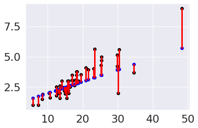
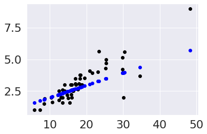
To examine these, we can plot them on the data:

plt.scatter(tips_X_test,tips_y_test, color='black')
plt.scatter(tips_X_test,tips_y_pred, color='blue')

[plt.plot([x,x],[yp,yt], color='red', linewidth=3)
         for x, yp, yt in zip(tips_X_test, tips_y_pred,tips_y_test)];

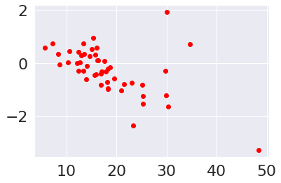
We can plot them as a scatter plot as well.

tips_residuals = tips_y_pred - tips_y_test
plt.scatter(tips_X_test,tips_residuals, color='red')

<matplotlib.collections.PathCollection at 0x7fb7e2feccd0>

One thing we notice is that the residuals are smaller for some values of the total_bill and larger for others. This suggests that there is more information left. A good fit, would have residuals that are evenly distributed, not correlated with the feature(s) in this case, the total bill.

21.2. Polynomial regression#

Polynomial regression is still a linear problem. Linear regression solves for the $\beta_i$ for a $d$ dimensional problem.

\[ y = \beta_0 + \beta_1 x_1 + \ldots + \beta_d x_d = \sum_i^d \beta_i x_i\]

Quadratic regression solves for

\[ y = \beta_0 + \sum_i^d \beta_i x_i$ + \sum_j^d \sum_i^d \beta_{d+i} x_i x_j + \sum_i^d x_i^2$ \]

This is still a linear problem, we can create a new $X$ matrix that has the polynomial values of each feature and solve for more $\beta$ values.

We use a transformer object, which works similarly to the estimators, but does not use targets. First, we instantiate.

poly = PolynomialFeatures(include_bias=False)

Then we apply it

tips_X2_train = poly.fit_transform(tips_X_train)
tips_X2_test = poly.fit_transform(tips_X_test)

We can see wht it did by looking at the shape.

tips_X_train.shape, tips_X2_train.shape

((195, 1), (195, 2))

tips_X2_train[:5,1]

array([ 722.5344, 1067.9824,  320.0521,  419.8401, 2320.3489])

tips_X_train[:5]

array([[26.88],
       [32.68],
       [17.89],
       [20.49],
       [48.17]])

tips_X2_train[:5,0]

array([26.88, 32.68, 17.89, 20.49, 48.17])

Now, we can fit a linear model on this data, which learns a weight for the data and it’s squared value.

regr2_tips = linear_model.LinearRegression()
regr2_tips.fit(tips_X2_train,tips_y_train)
tips2_y_pred = regr2_tips.predict(tips_X2_test)

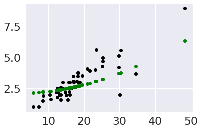
Then we can plot it.

plt.scatter(tips_X_test,tips_y_test, color='black')
plt.scatter(tips_X_test,tips_y_pred, color='blue')
plt.scatter(tips_X_test,tips2_y_pred, color='green')

<matplotlib.collections.PathCollection at 0x7fb7e0f63400>

We can see that this its somewhat better, the residuals are more uniformly distributed, but it doesn’t look very nonlinear.
We will examine this further in the next step, but first we will drop the linear column to see the quadratic more clearly.

poly = PolynomialFeatures()

tips_Xq_train = poly.fit_transform(tips_X_train)[:,::2]
tips_Xq_test = poly.fit_transform(tips_X_test)[:,::2]

regr_qu_tips = linear_model.LinearRegression(fit_intercept=False)
regr_qu_tips.fit(tips_Xq_train,tips_y_train)
tips2_q_pred = regr_qu_tips.predict(tips_Xq_test)

plt.scatter(tips_X_test,tips_y_test, color='black')
plt.scatter(tips_X_test,tips2_q_pred, color='green')

<matplotlib.collections.PathCollection at 0x7fb7e0f35fd0>

Try it Yourself

How would you make it cubic? what about 4th dimension?

21.3. Examining Coefficients#

Now we can compare the coefficients. We saw above that the quadratic didn’t help much, so let’s look at those.

regr2_tips.coef_

array([ 9.70620903e-02, -4.18198822e-06])

The second parameter is very very small, so that explains why it didn’t change the fit much. We can use the features to figure out how important each feature is to the prediction. Large numbers strongly influence the prediction smaller ones influence it less.

regr_tips.coef_

array([0.0968534])

21.4. Sparse Regression#

An extreme is for some coefficients to be zero. The LASSO model, constrains some of the coefficients to be 0, so it learns simultanesouly how to combine the features to predict the target and which subset of the features to use.

Further Reading

For the mathermatical formulation see the sklearn User Guide Section on LASSO and the code in LASSO docs

Thinking Ahead

LASSO is not required for assignment 8, but is one way you could earn level 3. Here is a preview, but you can investigate it further on your own.

tips_lasso = linear_model.Lasso(alpha=.0025)
tips_lasso.fit(tips_all_X_train,tips_all_y_train)
tips_lasso_y_pred = tips_lasso.predict(tips_all_X_test,)
tips_lasso.score(tips_all_X_test,tips_all_y_test)

---------------------------------------------------------------------------
NameError                                 Traceback (most recent call last)
Input In [23], in <cell line: 2>()
      1 tips_lasso = linear_model.Lasso(alpha=.0025)
----> 2 tips_lasso.fit(tips_all_X_train,tips_all_y_train)
      3 tips_lasso_y_pred = tips_lasso.predict(tips_all_X_test,)
      4 tips_lasso.score(tips_all_X_test,tips_all_y_test)

NameError: name 'tips_all_X_train' is not defined

plt.scatter(tips_X_test,tips_y_test, color='black')
plt.scatter(tips_X_test,tips_y_pred, color='blue')
plt.scatter(tips_X_test,tips_lasso_y_pred, color='green')

---------------------------------------------------------------------------
NameError                                 Traceback (most recent call last)
Input In [24], in <cell line: 3>()
      1 plt.scatter(tips_X_test,tips_y_test, color='black')
      2 plt.scatter(tips_X_test,tips_y_pred, color='blue')
----> 3 plt.scatter(tips_X_test,tips_lasso_y_pred, color='green')

NameError: name 'tips_lasso_y_pred' is not defined

sum(tips_lasso.coef_ ==0)/len(tips_lasso.coef_)

---------------------------------------------------------------------------
AttributeError                            Traceback (most recent call last)
Input In [25], in <cell line: 1>()
----> 1 sum(tips_lasso.coef_ ==0)/len(tips_lasso.coef_)

AttributeError: 'Lasso' object has no attribute 'coef_'

tips_onehot.shape, tips_interacion.shape

---------------------------------------------------------------------------
NameError                                 Traceback (most recent call last)
Input In [26], in <cell line: 1>()
----> 1 tips_onehot.shape, tips_interacion.shape

NameError: name 'tips_onehot' is not defined

The transform changed our data from 10 columns to 55.

tips_interacion.head

---------------------------------------------------------------------------
NameError                                 Traceback (most recent call last)
Input In [27], in <cell line: 1>()
----> 1 tips_interacion.head

NameError: name 'tips_interacion' is not defined

21.5. Questions After Class#

21.5.1. When do we do regression?#

we do regresion, when we want to predict a continuous value

21.5.2. What should I look for in datasets to know whether a linear model or non-linear model is best?#

If you know a reason to choose one from domain knowledge, always use that. From data alone, a reasonable thing to do is to fit a linear model and then examine the residuals and use a more complex model if that makes sense.

21.5.3. How can we tell if a dataset is going to be useful through tweaking or is just not worth it?#

This is a very good question, but does not have a simple answer. In some cases, a moderate fit quality is enough, because there’s low risk of making errors. In other cases, a really high quality fit is required because of the risk.

Programming for Data Science at URI Fall 2021

Interpretting Regression

Contents

21. Interpretting Regression#

21.1. Examining Residuals#

21.2. Polynomial regression#

21.3. Examining Coefficients#

21.4. Sparse Regression#

21.5. Questions After Class#

21.5.1. When do we do regression?#

21.5.2. What should I look for in datasets to know whether a linear model or non-linear model is best?#

21.5.3. How can we tell if a dataset is going to be useful through tweaking or is just not worth it?#