5. Getting Started with Exploratory Data Analysis

Now we get to start actual data science!

Our goal this week is to explore the actual data, the values, in a dataset to get a basic idea of what is in the data.

Summarizing and Visualizing Data are very important

• People cannot interpret high dimensional or large samples quickly

• Important in EDA to help you make decisions about the rest of your analysis

• Important in how you report your results

• Summaries are similar calculations to performance metrics we will see later

• visualizations are often essential in debugging models

THEREFORE

• You have a lot of chances to earn summarize and visualize

• we will be picky when we assess if you earned them or not

import pandas as pd

5.1. Staying Organized

• See the new File structure section.

• Be sure to accept assignments and close the feedback PR if you will not work on them

5.2. Loading Data and Examining Structure

coffee_data_url = 'https://raw.githubusercontent.com/jldbc/coffee-quality-database/master/data/robusta_data_cleaned.csv'
coffee_df = pd.read_csv(coffee_data_url,index_col=0)

So far, we’ve loaded data in a few different ways and then we’ve examined DataFrames as a data structure, looking at what different attributes they have and what some of the methods are, and how to get data into them.

coffee_df.head(2)

	Species	Owner	Country.of.Origin	Farm.Name	Lot.Number	Mill	ICO.Number	Company	Altitude	Region	...	Color	Category.Two.Defects	Expiration	Certification.Body	Certification.Address	Certification.Contact	unit_of_measurement	altitude_low_meters	altitude_high_meters	altitude_mean_meters
1	Robusta	ankole coffee producers coop	Uganda	kyangundu cooperative society	NaN	ankole coffee producers	0	ankole coffee producers coop	1488	sheema south western	...	Green	2	June 26th, 2015	Uganda Coffee Development Authority	e36d0270932c3b657e96b7b0278dfd85dc0fe743	03077a1c6bac60e6f514691634a7f6eb5c85aae8	m	1488.0	1488.0	1488.0
2	Robusta	nishant gurjer	India	sethuraman estate kaapi royale	25	sethuraman estate	14/1148/2017/21	kaapi royale	3170	chikmagalur karnataka indua	...	NaN	2	October 31st, 2018	Specialty Coffee Association	ff7c18ad303d4b603ac3f8cff7e611ffc735e720	352d0cf7f3e9be14dad7df644ad65efc27605ae2	m	3170.0	3170.0	3170.0

2 rows × 43 columns

From here we can see a few sample values of most of the column and we can be sure that the data loaded correctly.

Try it Yourself

What other tools have we learned to examine a DataFrame and when might you use them?

We can also get more structural information with the info method.

More information on this can also be found in the dtypes attribute. Including that the type is the most general if there are multiple types in the column.

Hint

There is also a related select_dtypes method.

coffee_df.info()

<class 'pandas.core.frame.DataFrame'>
Int64Index: 28 entries, 1 to 28
Data columns (total 43 columns):
 #   Column                 Non-Null Count  Dtype  
---  ------                 --------------  -----  
 0   Species                28 non-null     object 
 1   Owner                  28 non-null     object 
 2   Country.of.Origin      28 non-null     object 
 3   Farm.Name              25 non-null     object 
 4   Lot.Number             6 non-null      object 
 5   Mill                   20 non-null     object 
 6   ICO.Number             17 non-null     object 
 7   Company                28 non-null     object 
 8   Altitude               25 non-null     object 
 9   Region                 26 non-null     object 
 10  Producer               26 non-null     object 
 11  Number.of.Bags         28 non-null     int64  
 12  Bag.Weight             28 non-null     object 
 13  In.Country.Partner     28 non-null     object 
 14  Harvest.Year           28 non-null     int64  
 15  Grading.Date           28 non-null     object 
 16  Owner.1                28 non-null     object 
 17  Variety                3 non-null      object 
 18  Processing.Method      10 non-null     object 
 19  Fragrance...Aroma      28 non-null     float64
 20  Flavor                 28 non-null     float64
 21  Aftertaste             28 non-null     float64
 22  Salt...Acid            28 non-null     float64
 23  Bitter...Sweet         28 non-null     float64
 24  Mouthfeel              28 non-null     float64
 25  Uniform.Cup            28 non-null     float64
 26  Clean.Cup              28 non-null     float64
 27  Balance                28 non-null     float64
 28  Cupper.Points          28 non-null     float64
 29  Total.Cup.Points       28 non-null     float64
 30  Moisture               28 non-null     float64
 31  Category.One.Defects   28 non-null     int64  
 32  Quakers                28 non-null     int64  
 33  Color                  26 non-null     object 
 34  Category.Two.Defects   28 non-null     int64  
 35  Expiration             28 non-null     object 
 36  Certification.Body     28 non-null     object 
 37  Certification.Address  28 non-null     object 
 38  Certification.Contact  28 non-null     object 
 39  unit_of_measurement    28 non-null     object 
 40  altitude_low_meters    25 non-null     float64
 41  altitude_high_meters   25 non-null     float64
 42  altitude_mean_meters   25 non-null     float64
dtypes: float64(15), int64(5), object(23)
memory usage: 9.6+ KB

5.3. Summary Statistics

Now, we can actually start to analyze the data itself.

The describe method provides us with a set of summary statistics that broadly describe the data overall.

coffee_df.describe()

	Number.of.Bags	Harvest.Year	Fragrance...Aroma	Flavor	Aftertaste	Salt...Acid	Bitter...Sweet	Mouthfeel	Uniform.Cup	Clean.Cup	Balance	Cupper.Points	Total.Cup.Points	Moisture	Category.One.Defects	Quakers	Category.Two.Defects	altitude_low_meters	altitude_high_meters	altitude_mean_meters
count	28.000000	28.000000	28.000000	28.000000	28.000000	28.000000	28.000000	28.000000	28.000000	28.000000	28.000000	28.000000	28.000000	28.000000	28.000000	28.0	28.000000	25.00000	25.000000	25.000000
mean	168.000000	2013.964286	7.702500	7.630714	7.559643	7.657143	7.675714	7.506786	9.904286	9.928214	7.541786	7.761429	80.868929	0.065714	2.964286	0.0	1.892857	1367.60000	1387.600000	1377.600000
std	143.226317	1.346660	0.296156	0.303656	0.342469	0.261773	0.317063	0.725152	0.238753	0.211030	0.526076	0.330507	2.441233	0.058464	12.357280	0.0	2.601129	838.06205	831.884207	833.980216
min	1.000000	2012.000000	6.750000	6.670000	6.500000	6.830000	6.670000	5.080000	9.330000	9.330000	5.250000	6.920000	73.750000	0.000000	0.000000	0.0	0.000000	40.00000	40.000000	40.000000
25%	1.000000	2013.000000	7.580000	7.560000	7.397500	7.560000	7.580000	7.500000	10.000000	10.000000	7.500000	7.580000	80.170000	0.000000	0.000000	0.0	0.000000	795.00000	795.000000	795.000000
50%	170.000000	2014.000000	7.670000	7.710000	7.670000	7.710000	7.750000	7.670000	10.000000	10.000000	7.670000	7.830000	81.500000	0.100000	0.000000	0.0	1.000000	1095.00000	1200.000000	1100.000000
75%	320.000000	2015.000000	7.920000	7.830000	7.770000	7.830000	7.830000	7.830000	10.000000	10.000000	7.830000	7.920000	82.520000	0.120000	0.000000	0.0	2.000000	1488.00000	1488.000000	1488.000000
max	320.000000	2017.000000	8.330000	8.080000	7.920000	8.000000	8.420000	8.250000	10.000000	10.000000	8.000000	8.580000	83.750000	0.130000	63.000000	0.0	9.000000	3170.00000	3170.000000	3170.000000

From this, we can draw several conclusions. FOr example straightforward ones like:

• the smallest number of bags rated is 1 and at least 25% of the coffees rates only had 1 bag

• the first ratings included were 2012 and last in 2017 (min & max)

• the mean Mouthfeel was 7.5

• Category One defects are not very common ( the 75th% is 0)

Or more nuanced ones that compare across variables like

• the raters scored coffee higher on Uniformity.Cup and Clean.Cup than other scores (mean score; only on the ones that seem to have a scale of up to 8/10)

• the coffee varied more in Mouthfeel and Balance that most other scores (the std; only on the ones that seem to have a scale of of up to 8/10)

• there are 3 ratings with no altitude (count of other variables is 28; alt is 25

And these all give us a sense of the values and the distribution or spread fo the data in each column.

We can use the descriptive statistics on individual columns as well.

coffee_df['Balance'].describe()

count    28.000000
mean      7.541786
std       0.526076
min       5.250000
25%       7.500000
50%       7.670000
75%       7.830000
max       8.000000
Name: Balance, dtype: float64

To dig in on what the quantiles really mean, we can compute one manually.

First, we sort the data, then for the 25%, we select the point in index 6 because becaues there are 28 values.

balance_sorted = coffee_df['Balance'].sort_values().values

What value of x to pick out 25%

x = 6
balance_sorted[x]

7.5

further reading

On the documentation page for describe the “ See Also” shows the links to the documentation of most of the individual functions. This is a good way to learn about other things, or find something when you are not quite sure what it would be named. Go to a function thats similar to what you want and then look at the related functions.

We can also extract each of the statistics that the describe method calculates individually, by name. The quantiles are tricky, we cannot just .25%() to get the 25% percentile, we have to use the quantile method and pass it a value between 0 and 1.

coffee_df['Flavor'].quantile(.8)

7.83

Calculate the mean of Aftertaste

coffee_df['Aftertaste'].mean()

7.559642857142856

5.4. Describing Nonnumerical Variables

There are different columns in the describe than the the whole dataset:

coffee_df.columns

Index(['Species', 'Owner', 'Country.of.Origin', 'Farm.Name', 'Lot.Number',
       'Mill', 'ICO.Number', 'Company', 'Altitude', 'Region', 'Producer',
       'Number.of.Bags', 'Bag.Weight', 'In.Country.Partner', 'Harvest.Year',
       'Grading.Date', 'Owner.1', 'Variety', 'Processing.Method',
       'Fragrance...Aroma', 'Flavor', 'Aftertaste', 'Salt...Acid',
       'Bitter...Sweet', 'Mouthfeel', 'Uniform.Cup', 'Clean.Cup', 'Balance',
       'Cupper.Points', 'Total.Cup.Points', 'Moisture', 'Category.One.Defects',
       'Quakers', 'Color', 'Category.Two.Defects', 'Expiration',
       'Certification.Body', 'Certification.Address', 'Certification.Contact',
       'unit_of_measurement', 'altitude_low_meters', 'altitude_high_meters',
       'altitude_mean_meters'],
      dtype='object')

coffee_df.describe().columns

Index(['Number.of.Bags', 'Harvest.Year', 'Fragrance...Aroma', 'Flavor',
       'Aftertaste', 'Salt...Acid', 'Bitter...Sweet', 'Mouthfeel',
       'Uniform.Cup', 'Clean.Cup', 'Balance', 'Cupper.Points',
       'Total.Cup.Points', 'Moisture', 'Category.One.Defects', 'Quakers',
       'Category.Two.Defects', 'altitude_low_meters', 'altitude_high_meters',
       'altitude_mean_meters'],
      dtype='object')

We can get the prevalence of each one with value_counts

coffee_df['Color'].value_counts()

Green           20
Blue-Green       3
Bluish-Green     2
None             1
Name: Color, dtype: int64

Try it Yourself

Note value_counts does not count the NaN values, but count counts all of the not missing values and the shape of the DataFrame is the total number of rows. How can you get the number of missing Colors?

Describe only operates on the numerical columns, but we might want to know about the others. We can get the number of each value with value_counts

coffee_df['Country.of.Origin'].value_counts()

India            13
Uganda           10
United States     2
Ecuador           2
Vietnam           1
Name: Country.of.Origin, dtype: int64

We can get the name of the most common country out of this Series using idmax

coffee_df['Country.of.Origin'].value_counts().idxmax()

'India'

Or see only how many different values with the related:

coffee_df['Country.of.Origin'].nunique()

5

We can also use the mode function, which works on both numerical or nonnumerical

coffee_df['Country.of.Origin'].mode()

0    India
Name: Country.of.Origin, dtype: object

5.5. Basic Plotting

Pandas give us basic plotting capability built right into DataFrames.

coffee_df['Country.of.Origin'].value_counts().plot()

<AxesSubplot: >

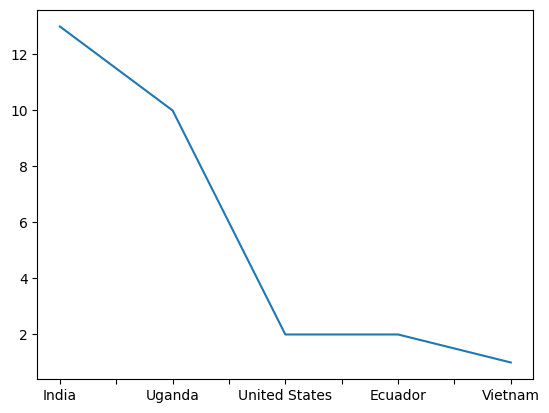
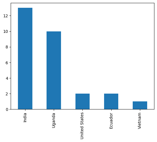
It defaults to a line graph, which is not very informative in this case, so we can use the kind parameter to change it to a bar graph.

coffee_df['Country.of.Origin'].value_counts().plot(kind='bar')

<AxesSubplot: >

5.6. Matching Questions to Summary Statistics

When we brainstorm more questions that we can answer with summary statistics or that we might want to ask of this data, the ones that come to mind are often actually dependent on two variables. For example are two scores correlated? or what country has the highest rated coffe on Flavor?

We’ll come back to more detailed questions like this on Friday, but to start we can look at how numerical variables vary by categorical (nonnumerical) variables by grouping the data.

Above we saw which country had the most ratings (remember one row is one rating), but what if we wanted to see the mean number of bags per country?

coffee_df.groupby('Country.of.Origin')['Number.of.Bags'].mean()

Country.of.Origin
Ecuador            1.000000
India            230.076923
Uganda           160.900000
United States     50.500000
Vietnam            1.000000
Name: Number.of.Bags, dtype: float64

Important

This data is only about coffee that was rated by a particular agency it is not economic data, so we cannot, for example conclude which country produces the amount of data. If we had economic dataset, a Number.of.Bags columns’s mean would tell us exactly that, but the context of the dataset defines what a row means and therefore how we can interpret the every single statistic we calculate.

5.7. Questions after class

5.7.1. Can arrays be used in Jupyter Notebook?

Jupyter runs a fully powered python interpreter, so all python can work inside it.

5.7.1.1. why did coffee_df[‘Country.of.Origin’].max() say vietnam?

That applies a the max function to the 'Country.of.Origin' column, without counting how many times the values occur.

5.7.1.2. Why, in the groupby function the first column is in between parenthesis nd the second one between brackets?

The inside parenthesis is the parameter of the groupby function, we could instead do it this way:

coffee_grouped = coffee_df.groupby('Country.of.Origin')

Then we can use coffee_grouped for different things

coffee_grouped.describe()

	Number.of.Bags								Harvest.Year		...	altitude_high_meters		altitude_mean_meters
	count	mean	std	min	25%	50%	75%	max	count	mean	...	75%	max	count	mean	std	min	25%	50%	75%	max
Country.of.Origin
Ecuador	2.0	1.000000	0.000000	1.0	1.00	1.0	1.00	1.0	2.0	2016.000000	...	40.00	40.0	1.0	40.000000	NaN	40.0	40.00	40.0	40.00	40.0
India	13.0	230.076923	110.280296	1.0	140.00	300.0	320.00	320.0	13.0	2014.384615	...	1500.00	3170.0	12.0	1421.666667	1021.022957	750.0	750.00	1000.0	1500.00	3170.0
Uganda	10.0	160.900000	163.690392	1.0	2.25	160.0	320.00	320.0	10.0	2013.300000	...	1488.00	1745.0	10.0	1354.500000	220.042546	1095.0	1203.00	1308.5	1488.00	1745.0
United States	2.0	50.500000	70.003571	1.0	25.75	50.5	75.25	100.0	2.0	2013.000000	...	2448.75	3000.0	2.0	1897.500000	1559.170453	795.0	1346.25	1897.5	2448.75	3000.0
Vietnam	1.0	1.000000	NaN	1.0	1.00	1.0	1.00	1.0	1.0	2013.000000	...	NaN	NaN	0.0	NaN	NaN	NaN	NaN	NaN	NaN	NaN

5 rows × 160 columns

or as we did before

coffee_grouped['Number.of.Bags'].mean()

Country.of.Origin
Ecuador            1.000000
India            230.076923
Uganda           160.900000
United States     50.500000
Vietnam            1.000000
Name: Number.of.Bags, dtype: float64

The second one is to index (see last week’s notes for more on indexing) the DataFrame and pick out one column. It makes the DataFrame have fewer columns before applying mean to the whole object.

We could make a smaller DataFrame first, then group, then mean

coffee_country_bags_df= coffee_df[['Number.of.Bags','Country.of.Origin']]
coffee_country_bags_df.head()

	Number.of.Bags	Country.of.Origin
1	300	Uganda
2	320	India
3	300	India
4	320	Uganda
5	1	Uganda

There are two sets of square brackets because putting a comma it would try to index along rows with one and columns with the other, to select multiple in one dimension you need to pass a list.

type(['Number.of.Bags','Country.of.Origin'])

list

If you do not put square [] or curly {} brackets around items, Python implicitly treats them as if there are parenthesis()

type(('Number.of.Bags','Country.of.Origin'))

tuple

and tuples are treated separately .

coffee_country_bags_df.groupby('Country.of.Origin').mean()

	Number.of.Bags
Country.of.Origin
Ecuador	1.000000
India	230.076923
Uganda	160.900000
United States	50.500000
Vietnam	1.000000

5.7.1.3. A quick recap of how .info() counts non-null and dtype for each column would be great. Thanks!

above

5.7.1.4. Can you plot a graph that uses two columns in a dataset?

Yes, we will see that on Wednesday.

5.7.1.5. Are there any other data types as important as dataframes in pandas?

DataFrames are the main type provided by pandas, there are also Series which is conceptually a single column, groupby objects which is basically a list of (DataFrame,label) tuples, and some indexing, but all of these exist to support creating and operating on DataFrames.

5.7.1.6. Will we be utilizing any other packages /libraries mentioned than the ones for visualizing data that we talked about today?

We will use pandas for basic plots and seaborn for more advanced plots. There are other libraries for visualization like plotly for interactive plots, but those are more advanced than we need or for specialized use cases. However, the way these type of libraries are designed, is that the special use case ones are for when the basic ones do not do what you need and they often have common patterns.

5.7.1.7. When displaying two categories like we did at the end could you measure a different thing for each category? Like count for one and mean for the other?

Yes! We will likely not do this in class, but it is a small extension from what we have covered and uses the pandas aggregrate method.

Hint

This is expected for visualize level 3

5.7.1.8. How in depth will we go with graphing data and looking at it systemically to find patterns?

At some level, that is what we sill do for the rest of the semester. We will not cover everything there is to know about graphing, there are whole courses on data visualization. Most of the pattern-finding we will do is machine learning.

5.7.2. Assignment

5.7.2.1. For assignment 2, how do I find appropriate datasets online?

I collated the ones that I recommend on the datasets page. Then find something that is of interest to you.

5.7.2.2. How do you import a .py file from GitHub? Is there a way to do that without downloading it locally?

It does need to be local in order to import it as a module.

Ideally, you will work with all of your assignment repos locally either following the instructions in the notes from last class