Visualization
Contents
6. Visualization#
import pandas as pd
6.1. A note on viewing output#
When we create a variable and then put that on the last line of a cell, jupyter displays it.
name = 'sarah'
name
'sarah'
How it displays it depends on the type
type(name)
str
For a string, it uses print
print(name)
sarah
so this and the one above look the same. For objects that have a _repr_html_
method, jupyter uses that, and then your brownser uses html to render the object
in a more visually appealing way.
6.2. Review from Monday#
We will load the robusta data briefly again.
robusta_data_url = 'https://raw.githubusercontent.com/jldbc/coffee-quality-database/master/data/robusta_data_cleaned.csv'
Is the robusta coffee’s Mouthfeel or Aftertaste rated more consistently
robusta_df = pd.read_csv(robusta_data_url)
robusta_df.describe()
| Unnamed: 0 | Number.of.Bags | Harvest.Year | Fragrance...Aroma | Flavor | Aftertaste | Salt...Acid | Bitter...Sweet | Mouthfeel | Uniform.Cup | ... | Balance | Cupper.Points | Total.Cup.Points | Moisture | Category.One.Defects | Quakers | Category.Two.Defects | altitude_low_meters | altitude_high_meters | altitude_mean_meters | |
|---|---|---|---|---|---|---|---|---|---|---|---|---|---|---|---|---|---|---|---|---|---|
| count | 28.000000 | 28.000000 | 28.000000 | 28.000000 | 28.000000 | 28.000000 | 28.000000 | 28.000000 | 28.000000 | 28.000000 | ... | 28.000000 | 28.000000 | 28.000000 | 28.000000 | 28.000000 | 28.0 | 28.000000 | 25.00000 | 25.000000 | 25.000000 |
| mean | 14.500000 | 168.000000 | 2013.964286 | 7.702500 | 7.630714 | 7.559643 | 7.657143 | 7.675714 | 7.506786 | 9.904286 | ... | 7.541786 | 7.761429 | 80.868929 | 0.065714 | 2.964286 | 0.0 | 1.892857 | 1367.60000 | 1387.600000 | 1377.600000 |
| std | 8.225975 | 143.226317 | 1.346660 | 0.296156 | 0.303656 | 0.342469 | 0.261773 | 0.317063 | 0.725152 | 0.238753 | ... | 0.526076 | 0.330507 | 2.441233 | 0.058464 | 12.357280 | 0.0 | 2.601129 | 838.06205 | 831.884207 | 833.980216 |
| min | 1.000000 | 1.000000 | 2012.000000 | 6.750000 | 6.670000 | 6.500000 | 6.830000 | 6.670000 | 5.080000 | 9.330000 | ... | 5.250000 | 6.920000 | 73.750000 | 0.000000 | 0.000000 | 0.0 | 0.000000 | 40.00000 | 40.000000 | 40.000000 |
| 25% | 7.750000 | 1.000000 | 2013.000000 | 7.580000 | 7.560000 | 7.397500 | 7.560000 | 7.580000 | 7.500000 | 10.000000 | ... | 7.500000 | 7.580000 | 80.170000 | 0.000000 | 0.000000 | 0.0 | 0.000000 | 795.00000 | 795.000000 | 795.000000 |
| 50% | 14.500000 | 170.000000 | 2014.000000 | 7.670000 | 7.710000 | 7.670000 | 7.710000 | 7.750000 | 7.670000 | 10.000000 | ... | 7.670000 | 7.830000 | 81.500000 | 0.100000 | 0.000000 | 0.0 | 1.000000 | 1095.00000 | 1200.000000 | 1100.000000 |
| 75% | 21.250000 | 320.000000 | 2015.000000 | 7.920000 | 7.830000 | 7.770000 | 7.830000 | 7.830000 | 7.830000 | 10.000000 | ... | 7.830000 | 7.920000 | 82.520000 | 0.120000 | 0.000000 | 0.0 | 2.000000 | 1488.00000 | 1488.000000 | 1488.000000 |
| max | 28.000000 | 320.000000 | 2017.000000 | 8.330000 | 8.080000 | 7.920000 | 8.000000 | 8.420000 | 8.250000 | 10.000000 | ... | 8.000000 | 8.580000 | 83.750000 | 0.130000 | 63.000000 | 0.0 | 9.000000 | 3170.00000 | 3170.000000 | 3170.000000 |
8 rows × 21 columns
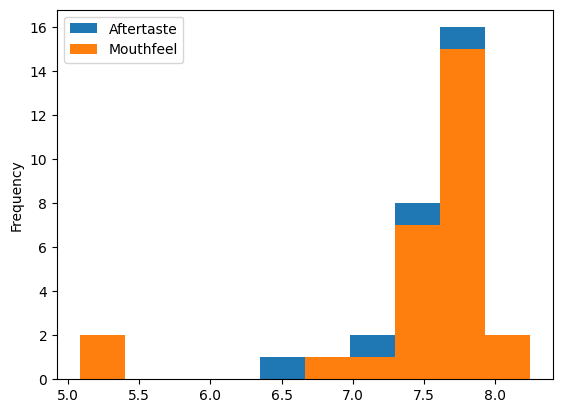
from the lower std we can see that Aftertaste is more consistently rated.
robusta_df[['Aftertaste','Mouthfeel']].plot(kind='hist')
<AxesSubplot: ylabel='Frequency'>
We can change the kind, for example to a Kernel Density Estimate. This approximates the distribution of the data, you can think of it rougly like a smoothed out histogram.
robusta_df[['Aftertaste','Mouthfeel']].plot(kind='kde')
<AxesSubplot: ylabel='Density'>
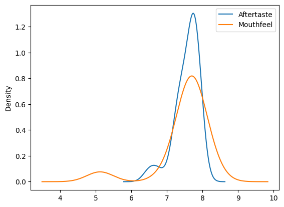
This version makess it more visually clear that the the Aftertaste is more consistently, but it also helps us see that that might not be the whole story. Both have a second smaller bump, so the overall std might not be the best measure.
Question from class
Why do we need two sets of brackets?
It tries to use them to index in multiple ways instead.
robusta_df['Aftertaste','Mouthfeel']
---------------------------------------------------------------------------
KeyError                                  Traceback (most recent call last)
File /opt/hostedtoolcache/Python/3.9.16/x64/lib/python3.9/site-packages/pandas/core/indexes/base.py:3803, in Index.get_loc(self, key, method, tolerance)
   3802 try:
-> 3803     return self._engine.get_loc(casted_key)
   3804 except KeyError as err:

File /opt/hostedtoolcache/Python/3.9.16/x64/lib/python3.9/site-packages/pandas/_libs/index.pyx:138, in pandas._libs.index.IndexEngine.get_loc()

File /opt/hostedtoolcache/Python/3.9.16/x64/lib/python3.9/site-packages/pandas/_libs/index.pyx:165, in pandas._libs.index.IndexEngine.get_loc()

File pandas/_libs/hashtable_class_helper.pxi:5745, in pandas._libs.hashtable.PyObjectHashTable.get_item()

File pandas/_libs/hashtable_class_helper.pxi:5753, in pandas._libs.hashtable.PyObjectHashTable.get_item()

KeyError: ('Aftertaste', 'Mouthfeel')

The above exception was the direct cause of the following exception:

KeyError                                  Traceback (most recent call last)
Cell In[9], line 1
----> 1 robusta_df['Aftertaste','Mouthfeel']

File /opt/hostedtoolcache/Python/3.9.16/x64/lib/python3.9/site-packages/pandas/core/frame.py:3805, in DataFrame.__getitem__(self, key)
   3803 if self.columns.nlevels > 1:
   3804     return self._getitem_multilevel(key)
-> 3805 indexer = self.columns.get_loc(key)
   3806 if is_integer(indexer):
   3807     indexer = [indexer]

File /opt/hostedtoolcache/Python/3.9.16/x64/lib/python3.9/site-packages/pandas/core/indexes/base.py:3805, in Index.get_loc(self, key, method, tolerance)
   3803     return self._engine.get_loc(casted_key)
   3804 except KeyError as err:
-> 3805     raise KeyError(key) from err
   3806 except TypeError:
   3807     # If we have a listlike key, _check_indexing_error will raise
   3808     #  InvalidIndexError. Otherwise we fall through and re-raise
   3809     #  the TypeError.
   3810     self._check_indexing_error(key)

KeyError: ('Aftertaste', 'Mouthfeel')
It tries to look for a multiindex, but we do not have one so it fails. THe second square brackets, makes it a list of names to use and pandas looks for them sequentially.
6.3. Comparing two datasets#
we’re going to work with the arabica data today, because it’s a little bigger and more interesting for plotting
arabica_data_url = 'https://raw.githubusercontent.com/jldbc/coffee-quality-database/master/data/arabica_data_cleaned.csv'
arabica_df = pd.read_csv(arabica_data_url,index_col=0)
It is mostly the same columns as the robusta data
arabica_df.columns
Index(['Species', 'Owner', 'Country.of.Origin', 'Farm.Name', 'Lot.Number',
       'Mill', 'ICO.Number', 'Company', 'Altitude', 'Region', 'Producer',
       'Number.of.Bags', 'Bag.Weight', 'In.Country.Partner', 'Harvest.Year',
       'Grading.Date', 'Owner.1', 'Variety', 'Processing.Method', 'Aroma',
       'Flavor', 'Aftertaste', 'Acidity', 'Body', 'Balance', 'Uniformity',
       'Clean.Cup', 'Sweetness', 'Cupper.Points', 'Total.Cup.Points',
       'Moisture', 'Category.One.Defects', 'Quakers', 'Color',
       'Category.Two.Defects', 'Expiration', 'Certification.Body',
       'Certification.Address', 'Certification.Contact', 'unit_of_measurement',
       'altitude_low_meters', 'altitude_high_meters', 'altitude_mean_meters'],
      dtype='object')
robusta_df.columns
Index(['Unnamed: 0', 'Species', 'Owner', 'Country.of.Origin', 'Farm.Name',
       'Lot.Number', 'Mill', 'ICO.Number', 'Company', 'Altitude', 'Region',
       'Producer', 'Number.of.Bags', 'Bag.Weight', 'In.Country.Partner',
       'Harvest.Year', 'Grading.Date', 'Owner.1', 'Variety',
       'Processing.Method', 'Fragrance...Aroma', 'Flavor', 'Aftertaste',
       'Salt...Acid', 'Bitter...Sweet', 'Mouthfeel', 'Uniform.Cup',
       'Clean.Cup', 'Balance', 'Cupper.Points', 'Total.Cup.Points', 'Moisture',
       'Category.One.Defects', 'Quakers', 'Color', 'Category.Two.Defects',
       'Expiration', 'Certification.Body', 'Certification.Address',
       'Certification.Contact', 'unit_of_measurement', 'altitude_low_meters',
       'altitude_high_meters', 'altitude_mean_meters'],
      dtype='object')
but it has a lot more rows
len(arabica_df) - len(robusta_df)
1283
arabica_df.shape, robusta_df.shape
((1311, 43), (28, 44))
6.4. Plotting in Python#
matplotlib: low level plotting tools
seaborn: high level plotting with opinionated defaults
ggplot: plotting based on the ggplot library in R.
Pandas and seaborn use matplotlib under the hood.
Seaborn and ggplot both assume the data is set up as a DataFrame. Getting started with seaborn is the simplest, so we’ll use that.
import seaborn as sns
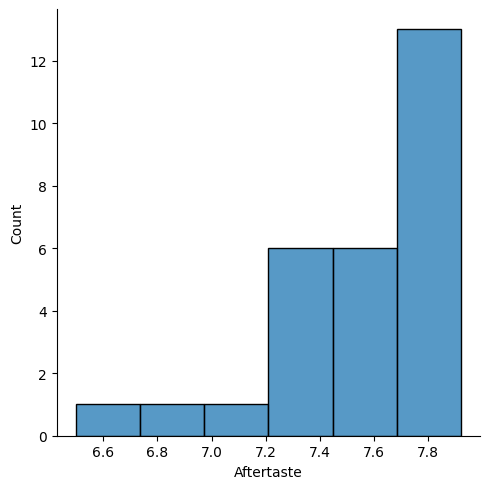
sns.displot(data = robusta_df, x='Aftertaste')
<seaborn.axisgrid.FacetGrid at 0x7f99bb81b340>
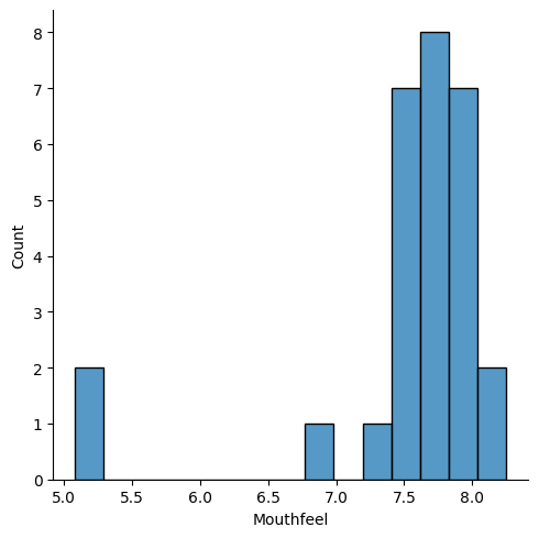
sns.displot(data = robusta_df, x='Mouthfeel')
<seaborn.axisgrid.FacetGrid at 0x7f99b020b370>
to plot these together with seaborn we have to transform the DataFrame, so we will see that next year.
6.4.1. how are flavor and balance related?#
sns.scatterplot(data=arabica_df,x='Flavor',y='Balance')
<AxesSubplot: xlabel='Flavor', ylabel='Balance'>
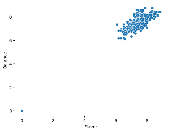
But now we have more power to investigate more relationships in the data.
sns.scatterplot(data=arabica_df,x='Flavor',y='Balance',hue='Color')
<AxesSubplot: xlabel='Flavor', ylabel='Balance'>
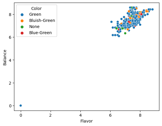
From this we can see that the color doesn’t appear to be related to the flavor or balance scores, but that the flavor and balacne are related.
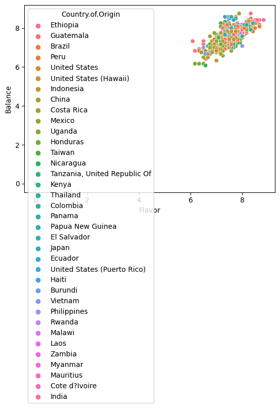
sns.scatterplot(data=arabica_df,x='Flavor',y='Balance',
                hue='Country.of.Origin')
<AxesSubplot: xlabel='Flavor', ylabel='Balance'>
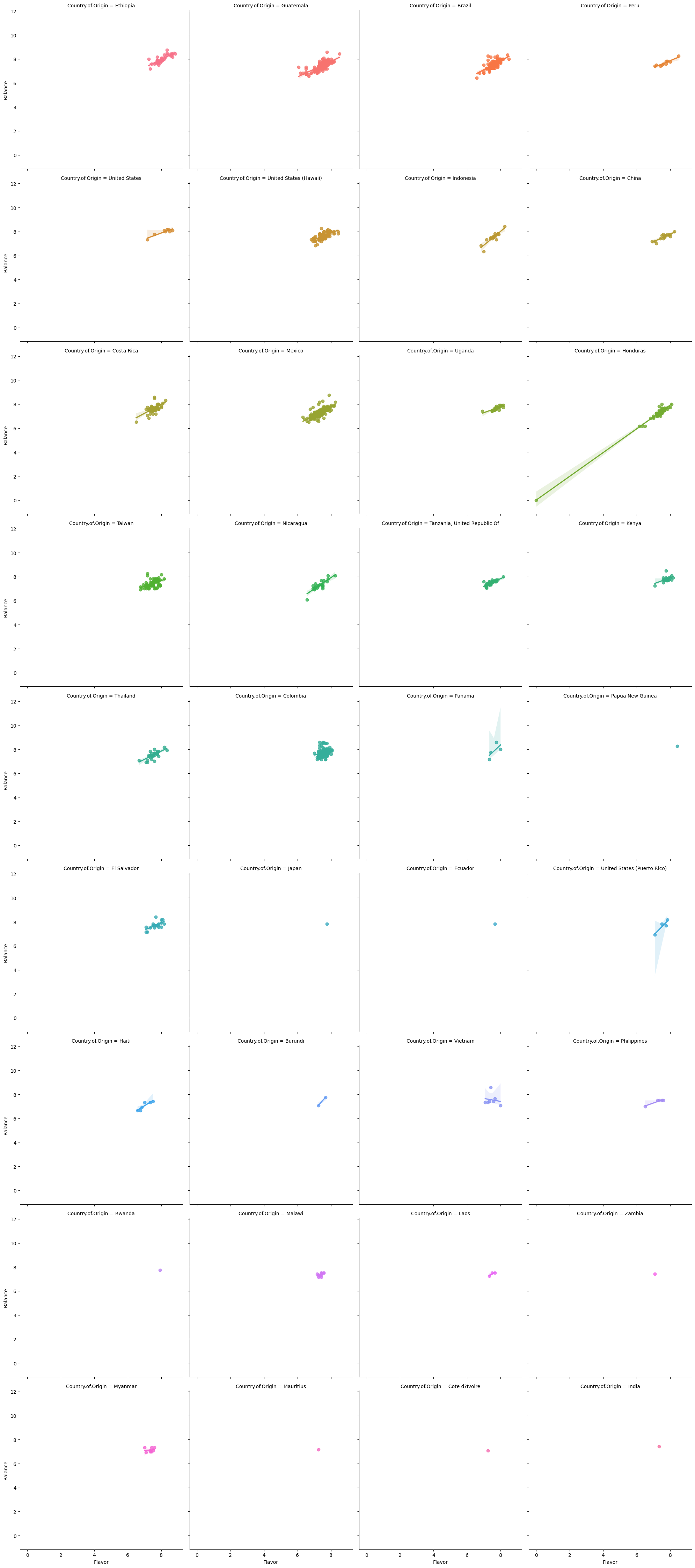
We can also break this apart. lmplot is a higher level plotting function so
it allows us to create grids of plots and by default also includes a regression
line.
sns.lmplot(data=arabica_df,x='Flavor',y='Balance',
                hue='Country.of.Origin',col='Country.of.Origin',
          col_wrap=4)
<seaborn.axisgrid.FacetGrid at 0x7f99afdfa0d0>
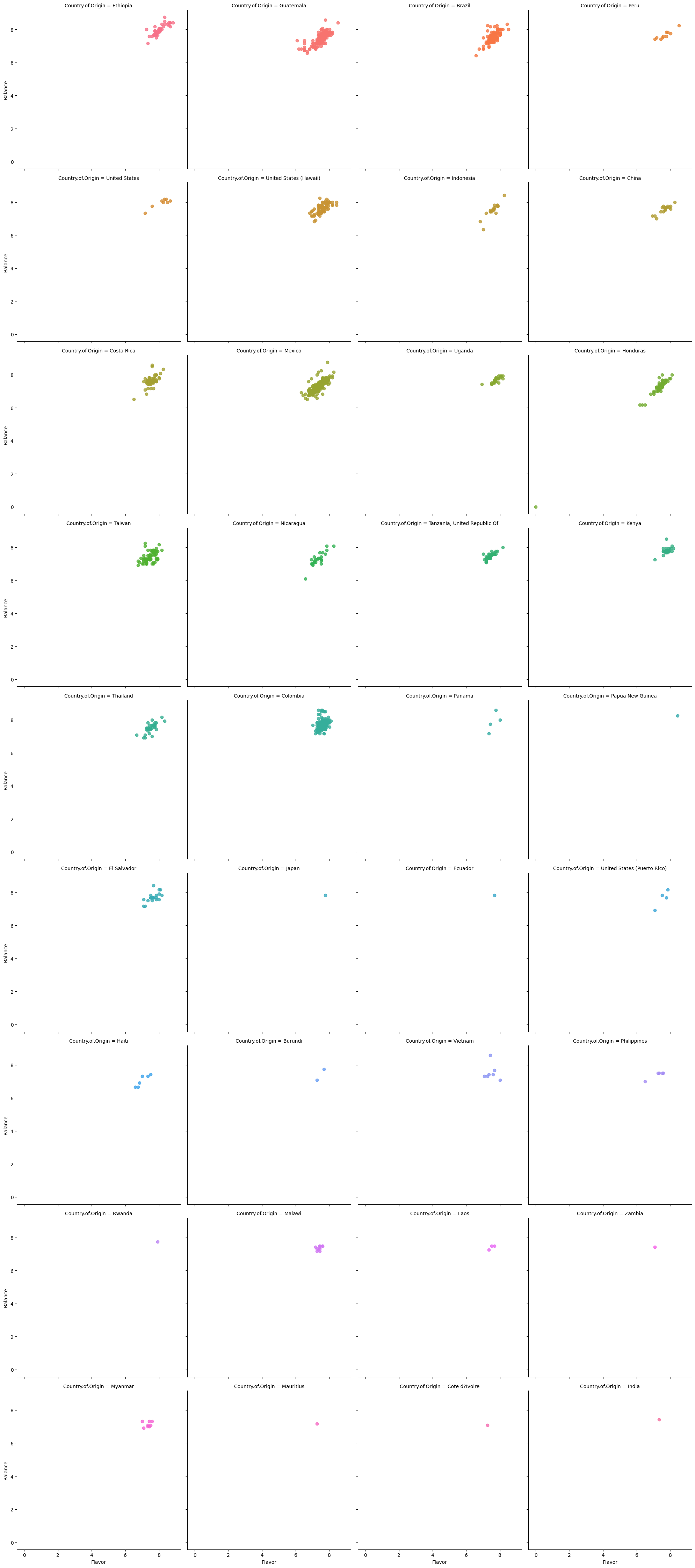
If we were not interested in the regression line, we could turn that off for now, with ,fit_reg=False.
sns.lmplot(data=arabica_df,x='Flavor',y='Balance',
                hue='Country.of.Origin',col='Country.of.Origin',
          col_wrap=4,fit_reg=False)
<seaborn.axisgrid.FacetGrid at 0x7f99a5b57eb0>
6.5. Things you want to know more about#
6.5.1. Things we will touch Friday#
more parameters and capabilities for seaborn
how to analyze a graph
6.5.2. Things that you could study for level 3#
The little details about the plot functions
More things that you can do with seaborn, like how to manipulate the scatterplots more
More ways to create unique plots and charts (we’ll give you a bit more depth but all the way here will be a level 3 task)
One thing I want to learn based on what’s learned so far is if we can compare graphs explicitly.
6.5.3. Things we will do later#
6.5.4. Graphing lines of best fit onto graphs (but not just linear models, quadratic or other types as well)#
We will learn how to fit models in general when we get to regression, but ultimately quadratic and other polynomial plots will also be a level 3 exploration you can do. We will get you to the point in class of all the pieces, but you will have to swap in some alternative parametrs
6.5.5. How to remove outliers or other data.#
When we saw indexing we got really close to this, and we will do more when we clean data next week.