
More EDA
Contents
7. More EDA#
import pandas as pd
import seaborn as sns
sns.set_theme(palette='colorblind')
arabica_data_url = 'https://raw.githubusercontent.com/jldbc/coffee-quality-database/master/data/arabica_data_cleaned.csv'
robusta_data_url = 'https://raw.githubusercontent.com/jldbc/coffee-quality-database/master/data/robusta_data_cleaned.csv'
coffee_df = pd.read_csv(arabica_data_url,index_col=0)
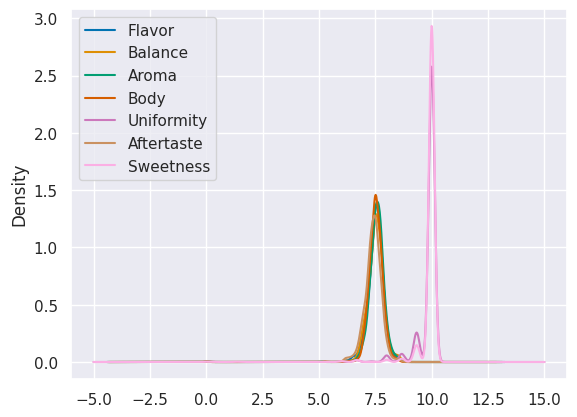
7.1. Which of the following is distributed most similarly to Sweetness?#
scores_of_interest = ['Flavor','Balance','Aroma','Body',
                      'Uniformity','Aftertaste','Sweetness']
We can answer this statistically, technically, but it will be easiest to do this looking ad a plot.
First step is to subset the data:
coffee_df[scores_of_interest].head(2)
| Flavor | Balance | Aroma | Body | Uniformity | Aftertaste | Sweetness | |
|---|---|---|---|---|---|---|---|
| 1 | 8.83 | 8.42 | 8.67 | 8.50 | 10.0 | 8.67 | 10.0 |
| 2 | 8.67 | 8.42 | 8.75 | 8.42 | 10.0 | 8.50 | 10.0 |
Then we produce a kde plot
coffee_df[scores_of_interest].plot(kind='kde')
<AxesSubplot: ylabel='Density'>
We could also do it with seaborn
sns.displot(data=coffee_df[scores_of_interest])
<seaborn.axisgrid.FacetGrid at 0x7f192e391370>
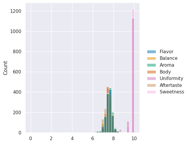
the default is not as helpful as using
sns.displot(data=coffee_df[scores_of_interest],kind='kde')
<seaborn.axisgrid.FacetGrid at 0x7f193276d1c0>
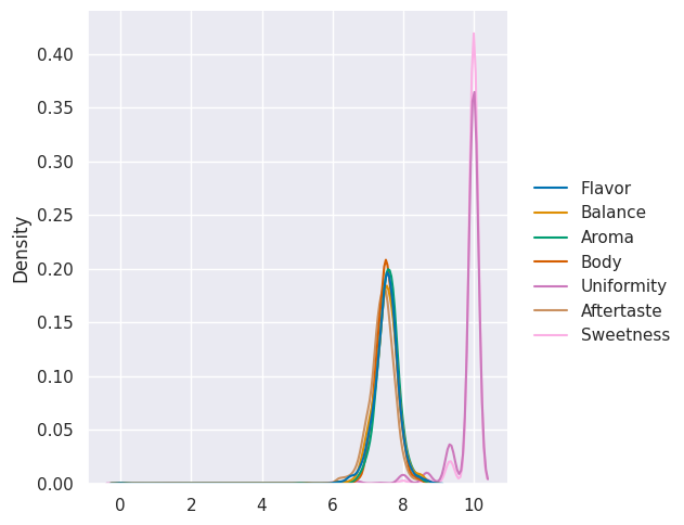
If we forget the parameter kind, we get its default value.
print('\n'.join(sns.displot.__doc__.split('\n')[5:10]))
``kind`` parameter selects the approach to use:

- :func:`histplot` (with ``kind="hist"``; the default)
- :func:`kdeplot` (with ``kind="kde"``)
- :func:`ecdfplot` (with ``kind="ecdf"``; univariate-only)
7.2. Summarizing with multiple variables#
So, we can summarize data now, but the summaries we have done so far have treated each variable one at a time. The most interesting patterns are in often in how multiple variables interact. We’ll do some modeling that looks at multivariate functions of data in a few weeks, but for now, we do a little more with summary statistics.
On Monday, we saw how to see how many reviews there were per country, using
total_per_country = coffee_df.groupby('Country.of.Origin')['Number.of.Bags'].sum()
What just happened?
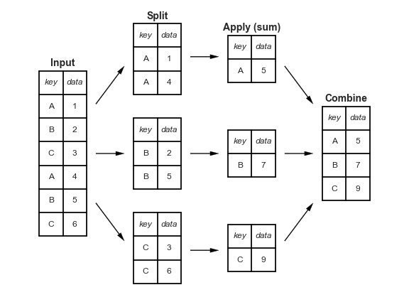
Groupby splits the whole dataframe into parts where each part has the same value for Country.of.Origin and then after that, we extracted the Number.of.Bags column, took the sum (within each separate group) and then put it all back together in one table (in this case, a Series becuase we picked one variable out)
7.2.1. How does Groupby Work?#
Important
This is more details with code examples on how the groupby works. If you want to run this code for yourself, use the download icon at the top right to download these notes as a notebook.
We can view this by saving the groupby object as a variable and exploring it.
country_grouped = coffee_df.groupby('Country.of.Origin')

country_grouped
<pandas.core.groupby.generic.DataFrameGroupBy object at 0x7f1932661910>
Trying to look at it without applying additional functions, just tells us the type. But, it’s iterable, so we can loop over.
for country,df in country_grouped:
    print(type(country), type(df))
<class 'str'> <class 'pandas.core.frame.DataFrame'>
<class 'str'> <class 'pandas.core.frame.DataFrame'>
<class 'str'> <class 'pandas.core.frame.DataFrame'>
<class 'str'> <class 'pandas.core.frame.DataFrame'>
<class 'str'> <class 'pandas.core.frame.DataFrame'>
<class 'str'> <class 'pandas.core.frame.DataFrame'>
<class 'str'> <class 'pandas.core.frame.DataFrame'>
<class 'str'> <class 'pandas.core.frame.DataFrame'>
<class 'str'> <class 'pandas.core.frame.DataFrame'>
<class 'str'> <class 'pandas.core.frame.DataFrame'>
<class 'str'> <class 'pandas.core.frame.DataFrame'>
<class 'str'> <class 'pandas.core.frame.DataFrame'>
<class 'str'> <class 'pandas.core.frame.DataFrame'>
<class 'str'> <class 'pandas.core.frame.DataFrame'>
<class 'str'> <class 'pandas.core.frame.DataFrame'>
<class 'str'> <class 'pandas.core.frame.DataFrame'>
<class 'str'> <class 'pandas.core.frame.DataFrame'>
<class 'str'> <class 'pandas.core.frame.DataFrame'>
<class 'str'> <class 'pandas.core.frame.DataFrame'>
<class 'str'> <class 'pandas.core.frame.DataFrame'>
<class 'str'> <class 'pandas.core.frame.DataFrame'>
<class 'str'> <class 'pandas.core.frame.DataFrame'>
<class 'str'> <class 'pandas.core.frame.DataFrame'>
<class 'str'> <class 'pandas.core.frame.DataFrame'>
<class 'str'> <class 'pandas.core.frame.DataFrame'>
<class 'str'> <class 'pandas.core.frame.DataFrame'>
<class 'str'> <class 'pandas.core.frame.DataFrame'>
<class 'str'> <class 'pandas.core.frame.DataFrame'>
<class 'str'> <class 'pandas.core.frame.DataFrame'>
<class 'str'> <class 'pandas.core.frame.DataFrame'>
<class 'str'> <class 'pandas.core.frame.DataFrame'>
<class 'str'> <class 'pandas.core.frame.DataFrame'>
<class 'str'> <class 'pandas.core.frame.DataFrame'>
<class 'str'> <class 'pandas.core.frame.DataFrame'>
<class 'str'> <class 'pandas.core.frame.DataFrame'>
<class 'str'> <class 'pandas.core.frame.DataFrame'>
We could manually compute things using the data structure, if needed, though using pandas functionality will usually do what we want. For example:
bag_total_dict = {}

for country,df in country_grouped:
    tot_bags =  df['Number.of.Bags'].sum()
    bag_total_dict[country] = tot_bags

pd.DataFrame.from_dict(bag_total_dict, orient='index',
                           columns = ['Number.of.Bags.Sum'])
| Number.of.Bags.Sum | |
|---|---|
| Brazil | 30534 |
| Burundi | 520 |
| China | 55 |
| Colombia | 41204 |
| Costa Rica | 10354 |
| Cote d?Ivoire | 2 |
| Ecuador | 1 |
| El Salvador | 4449 |
| Ethiopia | 11761 |
| Guatemala | 36868 |
| Haiti | 390 |
| Honduras | 13167 |
| India | 20 |
| Indonesia | 1658 |
| Japan | 20 |
| Kenya | 3971 |
| Laos | 81 |
| Malawi | 557 |
| Mauritius | 1 |
| Mexico | 24140 |
| Myanmar | 10 |
| Nicaragua | 6406 |
| Panama | 537 |
| Papua New Guinea | 7 |
| Peru | 2336 |
| Philippines | 259 |
| Rwanda | 150 |
| Taiwan | 1914 |
| Tanzania, United Republic Of | 3760 |
| Thailand | 1310 |
| Uganda | 3868 |
| United States | 361 |
| United States (Hawaii) | 833 |
| United States (Puerto Rico) | 71 |
| Vietnam | 10 |
| Zambia | 13 |
is the same as what we did before
7.3. Sorting DataFrames#
We saved the totals, so we can check what type that is.
type(total_per_country)
pandas.core.series.Series
It’s a pandas series, so we can use the sort_values method.
total_per_country.sort_values(ascending=False)
Country.of.Origin
Colombia                        41204
Guatemala                       36868
Brazil                          30534
Mexico                          24140
Honduras                        13167
Ethiopia                        11761
Costa Rica                      10354
Nicaragua                        6406
El Salvador                      4449
Kenya                            3971
Uganda                           3868
Tanzania, United Republic Of     3760
Peru                             2336
Taiwan                           1914
Indonesia                        1658
Thailand                         1310
United States (Hawaii)            833
Malawi                            557
Panama                            537
Burundi                           520
Haiti                             390
United States                     361
Philippines                       259
Rwanda                            150
Laos                               81
United States (Puerto Rico)        71
China                              55
India                              20
Japan                              20
Zambia                             13
Myanmar                            10
Vietnam                            10
Papua New Guinea                    7
Cote d?Ivoire                       2
Ecuador                             1
Mauritius                           1
Name: Number.of.Bags, dtype: int64
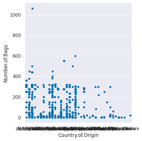
7.4. More plot types#
We can also look at the distributions
sns.catplot(data=coffee_df,x='Country.of.Origin',y='Number.of.Bags')
<seaborn.axisgrid.FacetGrid at 0x7f192e37b7f0>
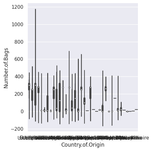
sns.catplot(data=coffee_df,x='Country.of.Origin',y='Number.of.Bags',
           kind='violin')
<seaborn.axisgrid.FacetGrid at 0x7f192e389130>
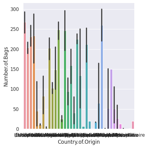
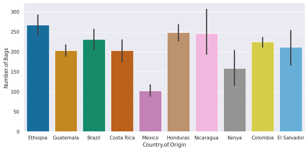
sns.catplot(data=coffee_df,x='Country.of.Origin',y='Number.of.Bags',
           kind='bar')
<seaborn.axisgrid.FacetGrid at 0x7f192ddef520>
7.5. How can we pick the top 10 countries out?#
total_per_country.sort_values(ascending=False)[:10]
Country.of.Origin
Colombia       41204
Guatemala      36868
Brazil         30534
Mexico         24140
Honduras       13167
Ethiopia       11761
Costa Rica     10354
Nicaragua       6406
El Salvador     4449
Kenya           3971
Name: Number.of.Bags, dtype: int64
type(total_per_country.sort_values(ascending=False)[:10])
pandas.core.series.Series
this is a series, but we can change it to a DataFrame with reset_index() this will also add a new index column but a side effect is that it becomes a DataFrame again
top_total_df = total_per_country.sort_values(ascending=False)[:10].reset_index()
top_total_df
| Country.of.Origin | Number.of.Bags | |
|---|---|---|
| 0 | Colombia | 41204 |
| 1 | Guatemala | 36868 |
| 2 | Brazil | 30534 |
| 3 | Mexico | 24140 |
| 4 | Honduras | 13167 |
| 5 | Ethiopia | 11761 |
| 6 | Costa Rica | 10354 |
| 7 | Nicaragua | 6406 |
| 8 | El Salvador | 4449 |
| 9 | Kenya | 3971 |
sns.catplot(data=top_total_df,x='Country.of.Origin',y='Number.of.Bags',
           kind='bar',aspect=2)
<seaborn.axisgrid.FacetGrid at 0x7f192dcf8670>
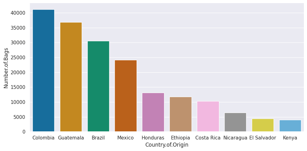
this got the number of countries fewer, bu they were still hard to read because they were small and still overlapping, so I added aspect=2 to make it 2x as wide as tall and give it more space. We can also use a similar strategy to pull out just these country names and get all the data for those.
top_countries = total_per_country.sort_values(ascending=False)[:10].index
coffee_df[coffee_df['Country.of.Origin'].isin(top_countries)].head(2)
| Species | Owner | Country.of.Origin | Farm.Name | Lot.Number | Mill | ICO.Number | Company | Altitude | Region | ... | Color | Category.Two.Defects | Expiration | Certification.Body | Certification.Address | Certification.Contact | unit_of_measurement | altitude_low_meters | altitude_high_meters | altitude_mean_meters | |
|---|---|---|---|---|---|---|---|---|---|---|---|---|---|---|---|---|---|---|---|---|---|
| 1 | Arabica | metad plc | Ethiopia | metad plc | NaN | metad plc | 2014/2015 | metad agricultural developmet plc | 1950-2200 | guji-hambela | ... | Green | 0 | April 3rd, 2016 | METAD Agricultural Development plc | 309fcf77415a3661ae83e027f7e5f05dad786e44 | 19fef5a731de2db57d16da10287413f5f99bc2dd | m | 1950.0 | 2200.0 | 2075.0 |
| 2 | Arabica | metad plc | Ethiopia | metad plc | NaN | metad plc | 2014/2015 | metad agricultural developmet plc | 1950-2200 | guji-hambela | ... | Green | 1 | April 3rd, 2016 | METAD Agricultural Development plc | 309fcf77415a3661ae83e027f7e5f05dad786e44 | 19fef5a731de2db57d16da10287413f5f99bc2dd | m | 1950.0 | 2200.0 | 2075.0 |
2 rows × 43 columns
I forgot the isin method in class and had to look that up, I more often need to filter by numerical columns or selecting a single value.
top_coffee_df = coffee_df[coffee_df['Country.of.Origin'].isin(top_countries)]
sns.catplot(data=top_coffee_df,x='Country.of.Origin',y='Number.of.Bags',
           kind='bar',aspect=2)
<seaborn.axisgrid.FacetGrid at 0x7f192db6ebb0>
top_coffee_df.info()
<class 'pandas.core.frame.DataFrame'>
Int64Index: 952 entries, 1 to 1312
Data columns (total 43 columns):
 #   Column                 Non-Null Count  Dtype
---  ------                 --------------  -----
 0   Species                952 non-null    object
 1   Owner                  945 non-null    object
 2   Country.of.Origin      952 non-null    object
 3   Farm.Name              694 non-null    object
 4   Lot.Number             205 non-null    object
 5   Mill                   760 non-null    object
 6   ICO.Number             908 non-null    object
 7   Company                789 non-null    object
 8   Altitude               833 non-null    object
 9   Region                 919 non-null    object
 10  Producer               812 non-null    object
 11  Number.of.Bags         952 non-null    int64
 12  Bag.Weight             952 non-null    object
 13  In.Country.Partner     952 non-null    object
 14  Harvest.Year           932 non-null    object
 15  Grading.Date           952 non-null    object
 16  Owner.1                945 non-null    object
 17  Variety                824 non-null    object
 18  Processing.Method      850 non-null    object
 19  Aroma                  952 non-null    float64
 20  Flavor                 952 non-null    float64
 21  Aftertaste             952 non-null    float64
 22  Acidity                952 non-null    float64
 23  Body                   952 non-null    float64
 24  Balance                952 non-null    float64
 25  Uniformity             952 non-null    float64
 26  Clean.Cup              952 non-null    float64
 27  Sweetness              952 non-null    float64
 28  Cupper.Points          952 non-null    float64
 29  Total.Cup.Points       952 non-null    float64
 30  Moisture               952 non-null    float64
 31  Category.One.Defects   952 non-null    int64
 32  Quakers                951 non-null    float64
 33  Color                  808 non-null    object
 34  Category.Two.Defects   952 non-null    int64
 35  Expiration             952 non-null    object
 36  Certification.Body     952 non-null    object
 37  Certification.Address  952 non-null    object
 38  Certification.Contact  952 non-null    object
 39  unit_of_measurement    952 non-null    object
 40  altitude_low_meters    830 non-null    float64
 41  altitude_high_meters   830 non-null    float64
 42  altitude_mean_meters   830 non-null    float64
dtypes: float64(16), int64(3), object(24)
memory usage: 327.2+ KB
sns.displot(top_coffee_df, x='Sweetness', kind='kde', col='Country.of.Origin',col_wrap=3)
<seaborn.axisgrid.FacetGrid at 0x7f192dfa65b0>
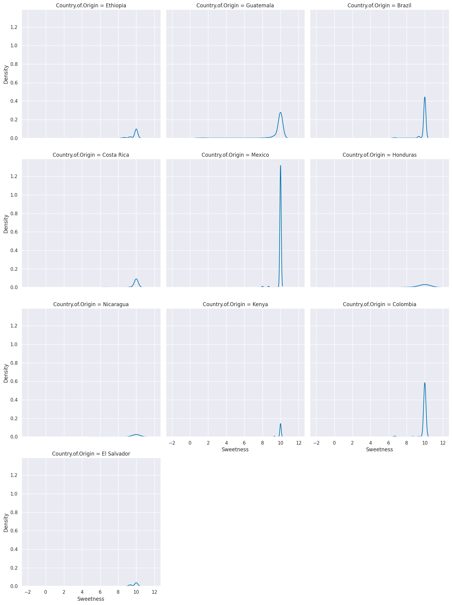
We’ll see next week how to manipulate the dataset so that we can plot multiple scores this way.
Variable types and data types Related but not the same.
7.6. General Plotting Ideas#
There are lots of type of plots, we saw the basic patterns of how to use them and we’ve used a few types, but we cannot (and do not need to) go through every single type. There are general patterns that you can use that will help you think about what type of plot you might want and help you understand them to be able to customize plots.
[Seaborn’s main goal is opinionated defaults and flexible customization](https://seaborn.pydata.org/tutorial/introduction.html#opinionated-defaults-and-flexible-customization
7.6.1. Anatomy of a figure#
First is the matplotlib structure of a figure. BOth pandas and seaborn and other plotting libraries use matplotlib. Matplotlib was used in visualizing the first Black hole.
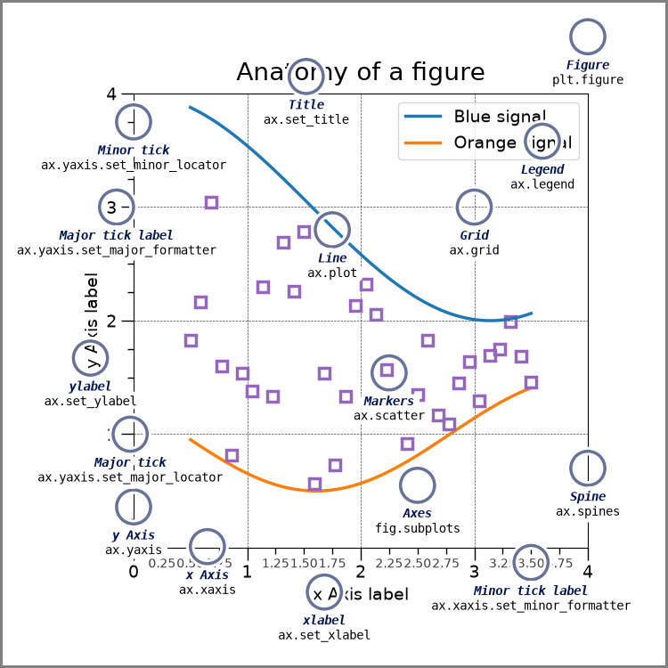
This is a lot of information, but these are good to know things. THe most important is the figure and the axes.
Try it Yourself
Make sure you can explain what is a figure and what are axes in your own words and why that distinction matters. Discuss in office hours if you are unsure.
that image was drawn with code and that page explains more.
7.6.2. Plotting Function types in Seaborn#
Seaborn has two levels or groups of plotting functions. Figure and axes. Figure level fucntions can plot with subplots.
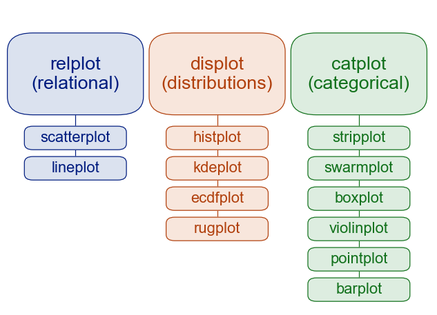
This is from thie overivew section of the official seaborn tutorial. It also includes a comparison of figure vs axes plotting.
The official introduction is also a good read.
7.6.3. More#
The seaborn gallery and matplotlib gallery are nice to look at too.
7.7. Styling Plots#
sns.set_theme()
sns.catplot(data=top_coffee_df,x='Country.of.Origin',y='Number.of.Bags',
           kind='bar',aspect=2)
<seaborn.axisgrid.FacetGrid at 0x7f192dac67f0>
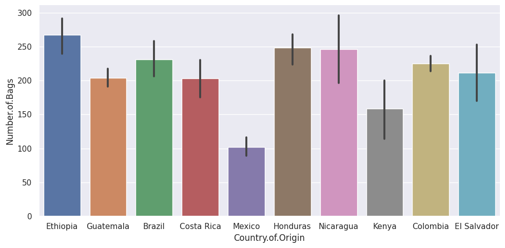
This by default styles the plots to be more visually appealing
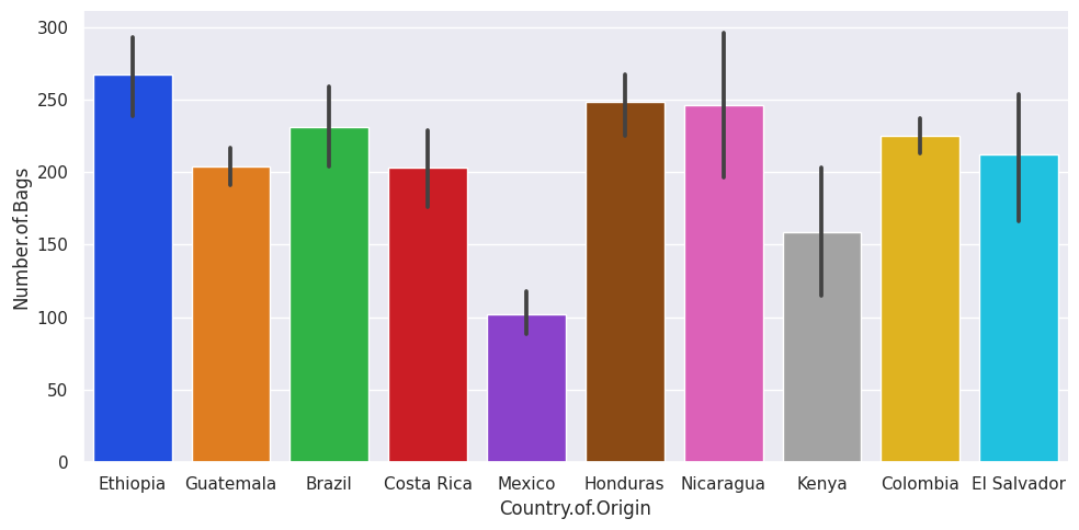
sns.set_theme(palette='colorblind')
sns.catplot(data=top_coffee_df,x='Country.of.Origin',y='Number.of.Bags',
           kind='bar',aspect=2)
<seaborn.axisgrid.FacetGrid at 0x7f192bb16400>
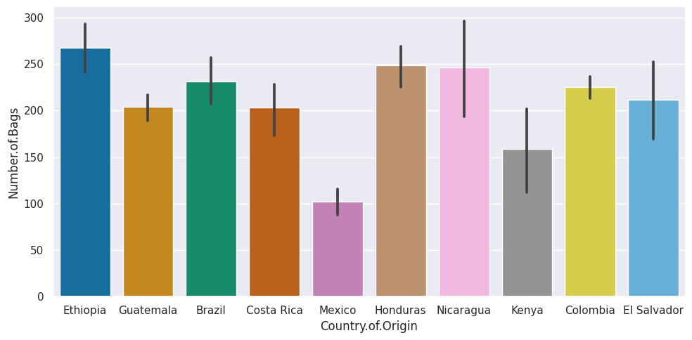
the colorblind palette is more distinguishable under a variety fo colorblindness types. for more
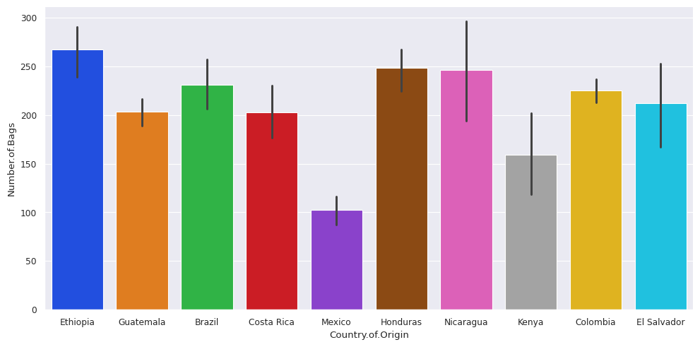
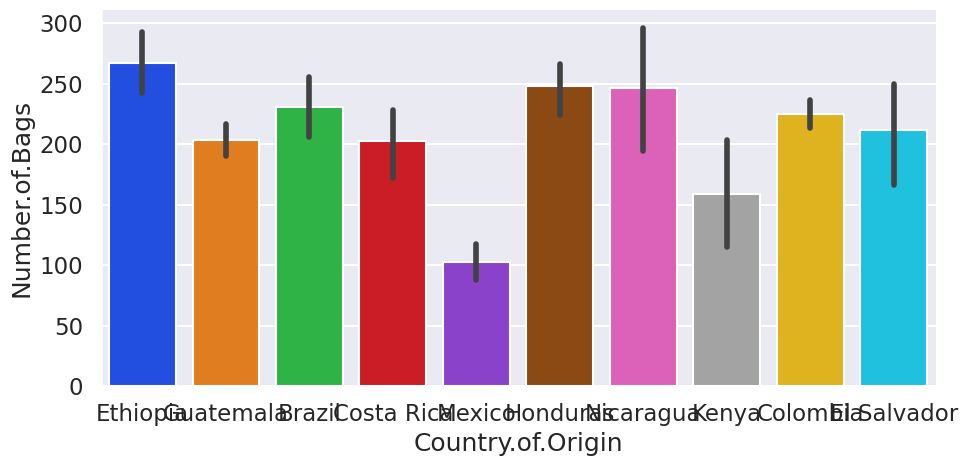
sns.set_theme(palette='bright')
sns.catplot(data=top_coffee_df,x='Country.of.Origin',y='Number.of.Bags',
           kind='bar',aspect=2)
<seaborn.axisgrid.FacetGrid at 0x7f1928adfee0>

Colorblind is a good default, but you can choose others that yo like more too.
to prepare plots for posters vs printing, etc you can use:
with sns.plotting_context('paper'):
    sns.catplot(data=top_coffee_df,x='Country.of.Origin',y='Number.of.Bags',
           kind='bar',aspect =2)
with sns.plotting_context('poster'):
    sns.catplot(data=top_coffee_df,x='Country.of.Origin',y='Number.of.Bags',
           kind='bar',aspect =2)
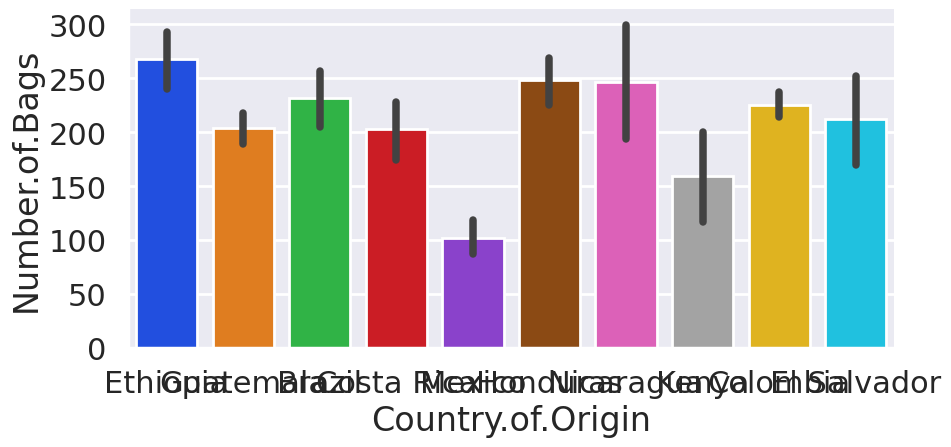
with sns.plotting_context('talk'):
    sns.catplot(data=top_coffee_df,x='Country.of.Origin',y='Number.of.Bags',
           kind='bar',aspect =2)
with sns.plotting_context('notebook'):
    sns.catplot(data=top_coffee_df,x='Country.of.Origin',y='Number.of.Bags',
           kind='bar',aspect =2)
It’s not perfect, but it gives you a good starting point.
7.8. More Practice#
Make a table thats total number of bags and mean and count of scored for each of the variables in the
scores_of_interestlist.Make a bar chart of the mean score for each variable
scores_of_interestgrouped by country.
7.9. Questions#
Note
Submit questions as Issues