
Sparse and Polynomial Regression
Contents
22. Sparse and Polynomial Regression#
import matplotlib.pyplot as plt
import seaborn as sns
import numpy as np
import pandas as pd
from sklearn import datasets, linear_model
from sklearn.metrics import mean_squared_error, r2_score
from sklearn.model_selection import cross_val_score
from sklearn.model_selection import train_test_split
from sklearn.preprocessing import PolynomialFeatures
sns.set_theme(font_scale=2,palette='colorblind')
22.1. Exmaining Residuals#
# Load the diabetes dataset
diabetes_X, diabetes_y = datasets.load_diabetes(return_X_y=True)
X_train,X_test, y_train,y_test = train_test_split(diabetes_X, diabetes_y ,
                         test_size=20,random_state=0)
regr_db = linear_model.LinearRegression()
regr_db.fit(X_train, y_train)
regr_db.score(X_test,y_test)
0.5195333332288746
regr_db.__dict__
{'fit_intercept': True,
 'copy_X': True,
 'n_jobs': None,
 'positive': False,
 'n_features_in_': 10,
 'coef_': array([ -32.30360126, -257.44019182,  513.32582416,  338.46035389,
        -766.84661714,  455.83564292,   92.5514199 ,  184.75080624,
         734.91009007,   82.72479583]),
 'rank_': 10,
 'singular_': array([1.95678408, 1.19959858, 1.08212757, 0.95268243, 0.79449825,
        0.76416914, 0.71267072, 0.64259342, 0.27343748, 0.0914504 ]),
 'intercept_': 152.391853606725}
y_pred = regr_db.predict(X_test)
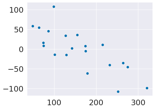
plt.scatter(y_test,y_pred)

plt.scatter(y_test, y_pred, color='black')
plt.plot(y_test, y_test, color='blue', linewidth=3)

# draw vertical lines frome each data point to its predict value
[plt.plot([x,x],[yp,yt], color='red', linewidth=3)
         for x, yp, yt in zip(y_test, y_pred,y_test)];

plt.xlabel('y_test')
plt.ylabel('y_pred')
Text(0, 0.5, 'y_pred')
Important
plotting the resiudals this way is okay for seeing how it did, but is not intepretted the same way, I’ve changed it for the correct interpretation. This says that there might not be enough information for high values to predict them, or maybe a better model could do it.
We can plot the residuals, more directly too:
test_df = pd.DataFrame(X_test,columns = ['x'+str(i) for i in range(len(X_test[0]))])
test_df['err'] = y_pred-y_test
x_df = test_df.melt(var_name = 'feature',id_vars=['err'])
x_df.head()
| err | feature | value | |
|---|---|---|---|
| 0 | -86.089041 | x0 | 0.019913 |
| 1 | 31.811770 | x0 | -0.012780 |
| 2 | 36.464326 | x0 | 0.038076 |
| 3 | 56.062302 | x0 | -0.012780 |
| 4 | 14.540509 | x0 | -0.023677 |
sns.relplot(data= x_df,x='value',col='feature', col_wrap=4,y='err')
<seaborn.axisgrid.FacetGrid at 0x7fbee4ec8820>
Here, we see that the residuals for most features are pretty uniform, but a few (eg the first one) are correlated to the feature value.
22.2. Polynomial regression#
Polynomial regression is still a linear problem. Linear regression solves for the \(\beta_i\) for a \(d\) dimensional problem.
Quadratic regression solves for
This is still a linear problem, we can create a new \(X\) matrix that has the polynomial values of each feature and solve for more \(\beta\) values.
We use a transformer object, which works similarly to the estimators, but does not use targets. First, we instantiate.
poly = PolynomialFeatures(include_bias=False,)
Then we can transform the data
X2_train = poly.fit_transform(X_train)
X2_train.shape
(422, 65)
X_train.shape
(422, 10)
regr_db2 = linear_model.LinearRegression()
regr_db2.fit(X2_train,y_train)
regr_db2.score(X2_test,y_test)
---------------------------------------------------------------------------
NameError                                 Traceback (most recent call last)
Cell In[12], line 3
      1 regr_db2 = linear_model.LinearRegression()
      2 regr_db2.fit(X2_train,y_train)
----> 3 regr_db2.score(X2_test,y_test)

NameError: name 'X2_test' is not defined
We see the performance is a little better, but let’s look at the residuals again.
X2_test = poly.transform(X_test)
y_pred2 = regr_db2.predict(X2_test)
regr_db2.coef_
array([ 2.26718871e+01, -2.84321941e+02,  4.77972133e+02,  3.55751429e+02,
       -1.05551594e+03,  7.64836015e+02,  1.92998441e+02,  1.29510126e+02,
        9.95077095e+02,  6.97824322e+01,  1.35199820e+03,  3.45185945e+03,
        1.47333609e+02, -6.34976797e+01, -3.44685551e+03, -1.39445637e+03,
        5.68431155e+03,  5.24944560e+03,  1.93320706e+03,  1.44078438e+03,
       -1.71687299e+00,  1.07459375e+03,  1.71895547e+03,  1.01185087e+04,
       -8.18260464e+03, -2.98856060e+03, -2.75793035e+03, -2.63196845e+03,
        4.87268727e+02,  3.31912403e+02,  2.57451083e+03, -5.38594465e+03,
        3.88190888e+03,  2.88432660e+03,  4.95180080e+02,  2.98317779e+03,
       -5.23610008e+02, -6.08039517e+01,  8.85704665e+03, -5.89220694e+03,
       -3.89995076e+03, -1.62903703e+03, -2.50355665e+03, -2.07339059e+03,
        9.56513316e+04, -1.35146919e+05, -8.45241707e+04, -4.18163194e+04,
       -8.84048804e+04, -6.63039722e+03,  5.00187584e+04,  5.43127248e+04,
        2.05139512e+04,  6.78912952e+04,  4.41920280e+03,  2.10042065e+04,
        2.61797171e+04,  3.74988567e+04,  5.16395623e+03,  1.12705277e+04,
        1.13915240e+04,  4.08084006e+03,  2.05240548e+04,  2.20132713e+03,
        1.91176349e+03])
test_df2 = pd.DataFrame(X2_test,columns = ['x'+str(i) for i in range(len(X2_test[0]))])
test_df2['err'] = y_pred2-y_test
x_df2 = test_df2.melt(var_name = 'feature',id_vars=['err'])
sns.relplot(data= x_df2,x='value',col='feature', col_wrap=4,y='err')
<seaborn.axisgrid.FacetGrid at 0x7fbee4e9c5b0>
From this we can see that most of these features do not vary much at all.
X2_test.shape
(20, 65)
22.3. Sparse Regression#
lasso = linear_model.Lasso()
lasso.fit(X_train,y_train)
Lasso()In a Jupyter environment, please rerun this cell to show the HTML representation or trust the notebook.
On GitHub, the HTML representation is unable to render, please try loading this page with nbviewer.org.
Lasso()
y_pred_lasso = lasso.predict(X_test)
lasso.coef_
array([  0.        ,  -0.        , 358.27705585,   9.71139556,
         0.        ,   0.        ,  -0.        ,   0.        ,
       309.50698469,   0.        ])
plt.scatter(y_test,y_pred_lasso-y_test)
<matplotlib.collections.PathCollection at 0x7fbe9a7ddd00>
lasso.score(X_test,y_test)
0.42249260665177746
regr_db.score(X_test,y_test)
0.5195333332288746
lassoa2 = linear_model.Lasso(.3)
lassoa2.fit(X_train,y_train)
Lasso(alpha=0.3)In a Jupyter environment, please rerun this cell to show the HTML representation or trust the notebook.
On GitHub, the HTML representation is unable to render, please try loading this page with nbviewer.org.
Lasso(alpha=0.3)
lassoa2.coef_
array([   0.        ,  -11.95340191,  500.51749129,  196.16550764,
         -0.        ,   -0.        , -118.56561325,    0.        ,
        435.84950435,    0.        ])
y_pred_lasso2 = lassoa2.predict(X_test)
plt.scatter(y_test,y_pred_lasso2-y_test)
<matplotlib.collections.PathCollection at 0x7fbe92038dc0>
lassoa2.score(X_test,y_test)
0.549634807596075
lassoa2.score(X_train,y_train)
0.47656951646350165
22.4. Combining them#
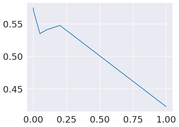
scores = []
alpha_vals = [1,.2,.1,.05,.001,.0005]
for alpha in alpha_vals:
    lasso2 = linear_model.Lasso(alpha)
    lasso2.fit(X2_train,y_train)
    scores.append(lasso2.score(X2_test,y_test))

plt.plot(alpha_vals,scores,)
/opt/hostedtoolcache/Python/3.9.16/x64/lib/python3.9/site-packages/sklearn/linear_model/_coordinate_descent.py:634: ConvergenceWarning: Objective did not converge. You might want to increase the number of iterations, check the scale of the features or consider increasing regularisation. Duality gap: 2.855e+05, tolerance: 2.501e+02
  model = cd_fast.enet_coordinate_descent(
/opt/hostedtoolcache/Python/3.9.16/x64/lib/python3.9/site-packages/sklearn/linear_model/_coordinate_descent.py:634: ConvergenceWarning: Objective did not converge. You might want to increase the number of iterations, check the scale of the features or consider increasing regularisation. Duality gap: 3.623e+05, tolerance: 2.501e+02
  model = cd_fast.enet_coordinate_descent(
[<matplotlib.lines.Line2D at 0x7fbe91fd8c40>]
lasso2 = linear_model.Lasso(.001)
lasso2.fit(X2_train,y_train)
lasso2.score(X2_test,y_test)
/opt/hostedtoolcache/Python/3.9.16/x64/lib/python3.9/site-packages/sklearn/linear_model/_coordinate_descent.py:634: ConvergenceWarning: Objective did not converge. You might want to increase the number of iterations, check the scale of the features or consider increasing regularisation. Duality gap: 2.855e+05, tolerance: 2.501e+02
  model = cd_fast.enet_coordinate_descent(
0.5700228082080702
lasso2.coef_
array([    7.2847557 ,  -265.03975714,   493.61070188,   349.64975297,
       -1615.37347603,  1235.50131986,   395.29739908,   180.43060963,
        1044.09619028,    85.9484476 ,  1459.71954915,  3939.7666462 ,
           0.        ,    62.32177997,    -0.        , -1303.73035699,
        1552.1397576 ,   104.05324926,  1360.85779052,   846.76212154,
          -0.        ,   981.75629416,  1279.46510906,     0.        ,
        -304.4411084 ,  1774.14494353,  -462.17132174,     0.        ,
           0.        ,   257.09550983,  2689.80253642,  -273.88698246,
          -0.        ,    -0.        ,     0.        ,   194.70180318,
          -0.        ,   -19.31963832,   499.65744841,     0.        ,
         409.75290934,    -0.        ,   206.38881023, -1512.15365558,
           0.        ,   964.06977666,     0.        , -3929.82319169,
          -0.        ,     0.        ,     0.        ,  -742.73744294,
           0.        ,  2350.36850741,     0.        ,     0.        ,
          -0.        ,   586.77368375,   538.26423584,   984.9462285 ,
       -1134.51637764,  1454.88328498,  2559.00186391,     0.        ,
        1590.6765506 ])
22.5. Tips example#
tips = sns.load_dataset("tips").dropna()
tips_X = tips['total_bill'].values
tips_X = tips_X[:,np.newaxis] # add an axis
tips_y = tips['tip']

tips_X_train,tips_X_test, tips_y_train, tips_y_test = train_test_split(
                     tips_X,
                     tips_y,
                     train_size=.8,
                     random_state=0)
In this example, we have one feature
regr_tips = linear_model.LinearRegression()
regr_tips.fit(tips_X_train,tips_y_train)
regr_tips.score(tips_X_test,tips_y_test)
0.5906895098589039
regr_tips.coef_, regr_tips.intercept_
(array([0.0968534]), 1.0285439454607272)
We can interpret this as that the expected tips is $1.02 + 9.7%.
tip_poly = PolynomialFeatures(include_bias=False,)
tips_X2_train = tip_poly.fit_transform(tips_X_train)
tips_X2_test = tip_poly.transform(tips_X_test)
regr2_tips = linear_model.LinearRegression()
regr2_tips.fit(tips_X2_train,tips_y_train)
regr2_tips.score(tips_X2_test,tips_y_test)
0.5907071399659565
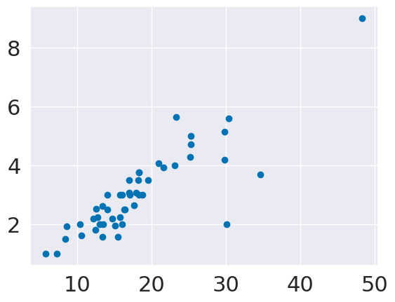
In this case, it doesn’t do any better, so the relationship is really linear.
plt.scatter(tips_X_test,tips_y_test)
<matplotlib.collections.PathCollection at 0x7fbe91f4fa90>
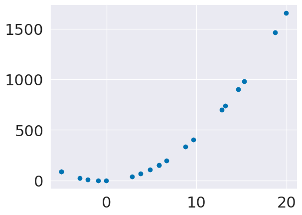
22.6. Toy example for visualization#
we’ll sample some random values for x and then add a coefficient to the value and the square
N = 20
slope = 3
sq = 4
sample_x = lambda num_smaples: np.random.normal(5,scale=10,size = num_smaples)
compute_y = lambda cx: slope*cx + sq*cx*cx
x_train = sample_x(N)[:,np.newaxis]
y_train = compute_y(x_train)

x_test = sample_x(N)[:,np.newaxis]
y_test = compute_y(x_test)
plt.scatter(x_train,y_train)
<matplotlib.collections.PathCollection at 0x7fbe91ec2130>
Now, we’ll transform, since this is one value
pf = PolynomialFeatures(include_bias=False,)
x2_train = pf.fit_transform(x_train,)
x2_test = pf.transform(x_test,)

plt.plot(x_train*x_train, x2_train[:,1])
[<matplotlib.lines.Line2D at 0x7fbe91e9f490>]
regr = linear_model.LinearRegression()
regr.fit(x2_train,y_train)

regr.score(x2_test,y_test)
1.0
regr.coef_
array([[3., 4.]])
y_pred = regr.predict(x2_test)
plt.scatter(x_test,y_pred)
<matplotlib.collections.PathCollection at 0x7fbe91dfed60>
