17. Classification with Naive Bayes

Note

This is typically not required but can fix issues. Mine was caused because I installed a package that reverted the version of my jupyter. This was the same problem that caused the notes to not render correctly.

The solution to this is to use environments more carefully.

%matplotlib inline

We’ll start with the same dataset as Monday.

import pandas as pd
import seaborn as sns
import numpy as np
from sklearn.model_selection import train_test_split
from sklearn.naive_bayes import GaussianNB
from sklearn import metrics
iris_df = sns.load_dataset('iris')

# dataset vars:
# ,
feature_vars = ['petal_width', 'sepal_length', 'sepal_width','petal_length']
target_var = 'species'
X_train, X_test, y_train, y_test = train_test_split(iris_df[feature_vars],iris_df[target_var],random_state=0)

Using the random_state makes it so that we get the same “random” set each type we run the code. see docs

X_train.head()

	petal_width	sepal_length	sepal_width	petal_length
61	1.5	5.9	3.0	4.2
92	1.2	5.8	2.6	4.0
112	2.1	6.8	3.0	5.5
2	0.2	4.7	3.2	1.3
141	2.3	6.9	3.1	5.1

iris_df.head(1)

	sepal_length	sepal_width	petal_length	petal_width	species
0	5.1	3.5	1.4	0.2	setosa

X_train.shape, iris_df.shape

((112, 4), (150, 5))

112/150

0.7466666666666667

We can see that we get ~75% of the samples in the training set by default. We could also see this from the docstring.

Again we will instantiate the object.

gnb = GaussianNB()

gnb.__dict__

{'priors': None, 'var_smoothing': 1e-09}

gnb.fit(X_train,y_train)

GaussianNB()

In a Jupyter environment, please rerun this cell to show the HTML representation or trust the notebook.
On GitHub, the HTML representation is unable to render, please try loading this page with nbviewer.org.

we fit the Gaussian Naive Bayes, it computes a mean \(\theta\) and variance \(\sigma\) and adds them to model parameters in attributes gnb.theta_, gnb.sigma_.

gnb.__dict__

{'priors': None,
 'var_smoothing': 1e-09,
 'classes_': array(['setosa', 'versicolor', 'virginica'], dtype='<U10'),
 'feature_names_in_': array(['petal_width', 'sepal_length', 'sepal_width', 'petal_length'],
       dtype=object),
 'n_features_in_': 4,
 'epsilon_': 3.2135586734693885e-09,
 'theta_': array([[0.24054054, 4.9972973 , 3.38918919, 1.45405405],
        [1.30882353, 5.91764706, 2.75882353, 4.19117647],
        [2.03902439, 6.66341463, 2.9902439 , 5.58292683]]),
 'var_': array([[0.01159971, 0.12242513, 0.14474799, 0.01978087],
        [0.0408045 , 0.2649827 , 0.11124568, 0.22139274],
        [0.06579417, 0.4071981 , 0.11453897, 0.30483046]]),
 'class_count_': array([37., 34., 41.]),
 'class_prior_': array([0.33035714, 0.30357143, 0.36607143])}

The attributes of the estimator object (gbn) describe the data (eg the class list) and the model’s parameters. The theta_ (\(\theta\)) represents the mean and the sigma_ (\(\sigma\)) represents the variance of the distributions.

Try it Yourself

Could you use what we learned about EDA to find the mean and variance of each feature for each species of flower?

Because the GaussianNB classifier calculates parameters that describe the assumed distribuiton of the data is is called a generative classifier. From a generative classifer, we can generate synthetic data that is from the distribution the classifer learned. If this data looks like our real data, then the model assumptions fit well.

Warning

the details of this math are not required understanding, but this describes the following block of code

Hint

to try understanding this block of code, try extracting pieces of it and running each piece individually. I built it up piece by piece adn then wrapped them all together.

To do this, we extract the mean and variance parameters from the model (gnb.theta_,gnb.sigma_) and zip them together to create an iterable object that in each iteration returns one value from each list (for th, sig in zip(gnb.theta_,gnb.sigma_)). We do this inside of a list comprehension and for each th,sig where th is from gnb.theta_ and sig is from gnb.sigma_ we use np.random.multivariate_normal to get 20 samples. In a general multivariate normal distribution the second parameter is actually a covariance matrix. This describes both the variance of each individual feature and the correlation of the features. Since Naive Bayes is Naive it assumes the features are independent or have 0 correlation. So, to create the matrix from the vector of variances we multiply by np.eye(4) which is the identity matrix or a matrix with 1 on the diagonal and 0 elsewhere. Finally we stack the groups for each species together with np.concatenate (like pd.concat but works on numpy objects and np.random.multivariate_normal returns numpy arrays not data frames) and put all of that in a DataFrame using the feature names as the columns.

Then we add a species column, by repeating each species 20 times [c]*N for c in gnb.classes_ and then unpack that into a single list instead of as list of lists.

N = 20
gnb_df = pd.DataFrame(np.concatenate([np.random.multivariate_normal(th, sig*np.eye(4),N)
         for th, sig in zip(gnb.var_,gnb.sigma_)]),
         columns = feature_vars)
gnb_df['species'] = [ci for cl in [[c]*N for c in gnb.classes_] for ci in cl]

---------------------------------------------------------------------------
AttributeError                            Traceback (most recent call last)
Cell In[12], line 3
      1 N = 20
      2 gnb_df = pd.DataFrame(np.concatenate([np.random.multivariate_normal(th, sig*np.eye(4),N)
----> 3          for th, sig in zip(gnb.var_,gnb.sigma_)]),
      4          columns = feature_vars)
      5 gnb_df['species'] = [ci for cl in [[c]*N for c in gnb.classes_] for ci in cl]

AttributeError: 'GaussianNB' object has no attribute 'sigma_'

sns.pairplot(data =gnb_df, hue='species')

---------------------------------------------------------------------------
NameError                                 Traceback (most recent call last)
Cell In[13], line 1
----> 1 sns.pairplot(data =gnb_df, hue='species')

NameError: name 'gnb_df' is not defined

Further Reading

There are other classifiers that use roughly the same model but don’t make the naive assumption. The more flexible is called Quadratic Discriminant Analysis.

• mathematical formulation for both

• QDA code

• LDA code

This one looks pretty close to the actual data. The biggest difference is that these data are all in uniformly circular-ish blobs and the ones above are not.
That means that the naive assumption doesn’t hold perfectly on this data.

sns.pairplot(data=iris_df,hue='species')

---------------------------------------------------------------------------
TypeError                                 Traceback (most recent call last)
Cell In[14], line 1
----> 1 sns.pairplot(data=iris_df,hue='species')

File /opt/hostedtoolcache/Python/3.9.16/x64/lib/python3.9/site-packages/seaborn/axisgrid.py:2148, in pairplot(data, hue, hue_order, palette, vars, x_vars, y_vars, kind, diag_kind, markers, height, aspect, corner, dropna, plot_kws, diag_kws, grid_kws, size)
   2146     diag_kws.setdefault("fill", True)
   2147     diag_kws.setdefault("warn_singular", False)
-> 2148     grid.map_diag(kdeplot, **diag_kws)
   2150 # Maybe plot on the off-diagonals
   2151 if diag_kind is not None:

File /opt/hostedtoolcache/Python/3.9.16/x64/lib/python3.9/site-packages/seaborn/axisgrid.py:1507, in PairGrid.map_diag(self, func, **kwargs)
   1505     plot_kwargs.setdefault("hue_order", self._hue_order)
   1506     plot_kwargs.setdefault("palette", self._orig_palette)
-> 1507     func(x=vector, **plot_kwargs)
   1508     ax.legend_ = None
   1510 self._add_axis_labels()

File /opt/hostedtoolcache/Python/3.9.16/x64/lib/python3.9/site-packages/seaborn/distributions.py:1717, in kdeplot(data, x, y, hue, weights, palette, hue_order, hue_norm, color, fill, multiple, common_norm, common_grid, cumulative, bw_method, bw_adjust, warn_singular, log_scale, levels, thresh, gridsize, cut, clip, legend, cbar, cbar_ax, cbar_kws, ax, **kwargs)
   1713 if p.univariate:
   1715     plot_kws = kwargs.copy()
-> 1717     p.plot_univariate_density(
   1718         multiple=multiple,
   1719         common_norm=common_norm,
   1720         common_grid=common_grid,
   1721         fill=fill,
   1722         color=color,
   1723         legend=legend,
   1724         warn_singular=warn_singular,
   1725         estimate_kws=estimate_kws,
   1726         **plot_kws,
   1727     )
   1729 else:
   1731     p.plot_bivariate_density(
   1732         common_norm=common_norm,
   1733         fill=fill,
   (...)
   1743         **kwargs,
   1744     )

File /opt/hostedtoolcache/Python/3.9.16/x64/lib/python3.9/site-packages/seaborn/distributions.py:996, in _DistributionPlotter.plot_univariate_density(self, multiple, common_norm, common_grid, warn_singular, fill, color, legend, estimate_kws, **plot_kws)
    993 if "x" in self.variables:
    995     if fill:
--> 996         artist = ax.fill_between(support, fill_from, density, **artist_kws)
    998     else:
    999         artist, = ax.plot(support, density, **artist_kws)

File /opt/hostedtoolcache/Python/3.9.16/x64/lib/python3.9/site-packages/matplotlib/__init__.py:1423, in _preprocess_data.<locals>.inner(ax, data, *args, **kwargs)
   1420 @functools.wraps(func)
   1421 def inner(ax, *args, data=None, **kwargs):
   1422     if data is None:
-> 1423         return func(ax, *map(sanitize_sequence, args), **kwargs)
   1425     bound = new_sig.bind(ax, *args, **kwargs)
   1426     auto_label = (bound.arguments.get(label_namer)
   1427                   or bound.kwargs.get(label_namer))

File /opt/hostedtoolcache/Python/3.9.16/x64/lib/python3.9/site-packages/matplotlib/axes/_axes.py:5367, in Axes.fill_between(self, x, y1, y2, where, interpolate, step, **kwargs)
   5365 def fill_between(self, x, y1, y2=0, where=None, interpolate=False,
   5366                  step=None, **kwargs):
-> 5367     return self._fill_between_x_or_y(
   5368         "x", x, y1, y2,
   5369         where=where, interpolate=interpolate, step=step, **kwargs)

File /opt/hostedtoolcache/Python/3.9.16/x64/lib/python3.9/site-packages/matplotlib/axes/_axes.py:5272, in Axes._fill_between_x_or_y(self, ind_dir, ind, dep1, dep2, where, interpolate, step, **kwargs)
   5268         kwargs["facecolor"] = \
   5269             self._get_patches_for_fill.get_next_color()
   5271 # Handle united data, such as dates
-> 5272 ind, dep1, dep2 = map(
   5273     ma.masked_invalid, self._process_unit_info(
   5274         [(ind_dir, ind), (dep_dir, dep1), (dep_dir, dep2)], kwargs))
   5276 for name, array in [
   5277         (ind_dir, ind), (f"{dep_dir}1", dep1), (f"{dep_dir}2", dep2)]:
   5278     if array.ndim > 1:

File /opt/hostedtoolcache/Python/3.9.16/x64/lib/python3.9/site-packages/numpy/ma/core.py:2360, in masked_invalid(a, copy)
   2332 def masked_invalid(a, copy=True):
   2333     """
   2334     Mask an array where invalid values occur (NaNs or infs).
   2335 
   (...)
   2357 
   2358     """
-> 2360     return masked_where(~(np.isfinite(getdata(a))), a, copy=copy)

TypeError: ufunc 'isfinite' not supported for the input types, and the inputs could not be safely coerced to any supported types according to the casting rule ''safe''

When we use the predict method, it uses those parameters to calculate the likelihood of the sample according to a Gaussian distribution (normal) for each class and then calculates the probability of the sample belonging to each class and returns the one with the highest probability.

y_pred = gnb.predict(X_test)

We can check the performance by comparing manually

sum(y_pred ==y_test)/len(y_test)

1.0

Or by scoring it.

gnb.score(X_test,y_test)

1.0

metrics.confusion_matrix(y_test,y_pred)

array([[13,  0,  0],
       [ 0, 16,  0],
       [ 0,  0,  9]])

17.1. Interpretting probabilities

gnb.predict_proba(X_test)

array([[2.05841140e-233, 1.23816844e-006, 9.99998762e-001],
       [1.76139943e-084, 9.99998414e-001, 1.58647449e-006],
       [1.00000000e+000, 1.48308613e-018, 1.73234612e-027],
       [6.96767669e-312, 5.33743814e-007, 9.99999466e-001],
       [1.00000000e+000, 9.33944060e-017, 1.22124682e-026],
       [4.94065646e-324, 6.57075840e-011, 1.00000000e+000],
       [1.00000000e+000, 1.05531886e-016, 1.55777574e-026],
       [2.45560284e-149, 7.80950359e-001, 2.19049641e-001],
       [4.01160627e-153, 9.10103555e-001, 8.98964447e-002],
       [1.46667004e-094, 9.99887821e-001, 1.12179234e-004],
       [5.29999917e-215, 4.59787449e-001, 5.40212551e-001],
       [4.93479766e-134, 9.46482991e-001, 5.35170089e-002],
       [5.23735688e-135, 9.98906155e-001, 1.09384481e-003],
       [4.97057521e-142, 9.50340361e-001, 4.96596389e-002],
       [9.11315109e-143, 9.87982897e-001, 1.20171030e-002],
       [1.00000000e+000, 7.81797826e-019, 1.29694954e-028],
       [3.86310964e-133, 9.87665084e-001, 1.23349155e-002],
       [2.27343573e-113, 9.99940331e-001, 5.96690955e-005],
       [1.00000000e+000, 1.80007196e-015, 9.14666201e-026],
       [1.00000000e+000, 1.30351394e-015, 8.42776899e-025],
       [4.66537803e-188, 1.18626155e-002, 9.88137385e-001],
       [1.02677291e-131, 9.92205279e-001, 7.79472050e-003],
       [1.00000000e+000, 6.61341173e-013, 1.42044069e-022],
       [1.00000000e+000, 9.98321355e-017, 3.50690661e-027],
       [2.27898063e-170, 1.61227371e-001, 8.38772629e-001],
       [1.00000000e+000, 2.29415652e-018, 2.54202512e-028],
       [1.00000000e+000, 5.99780345e-011, 5.24260178e-020],
       [1.62676386e-112, 9.99340062e-001, 6.59938068e-004],
       [2.23238199e-047, 9.99999965e-001, 3.47984452e-008],
       [1.00000000e+000, 1.95773682e-013, 4.10256723e-023],
       [3.52965800e-228, 1.15450262e-003, 9.98845497e-001],
       [3.20480410e-131, 9.93956330e-001, 6.04366979e-003],
       [1.00000000e+000, 1.14714843e-016, 2.17310302e-026],
       [3.34423817e-177, 8.43422262e-002, 9.15657774e-001],
       [5.60348582e-264, 1.03689515e-006, 9.99998963e-001],
       [7.48035097e-091, 9.99950155e-001, 4.98452400e-005],
       [1.00000000e+000, 1.80571225e-013, 1.83435499e-022],
       [8.97496247e-182, 5.65567226e-001, 4.34432774e-001]])

These are hard to interpret as is, one option is to plot them

# make the prbabilities into a dataframe labeled with classes & make the index a separate column
prob_df = pd.DataFrame(data = gnb.predict_proba(X_test), columns = gnb.classes_ ).reset_index()
# add the predictions
prob_df['predicted_species'] = y_pred
prob_df['true_species'] = y_test.values
# for plotting, make a column that combines the index & prediction
pred_text = lambda r: str( r['index']) + ',' + r['predicted_species']
prob_df['i,pred'] = prob_df.apply(pred_text,axis=1)
# same for ground truth
true_text = lambda r: str( r['index']) + ',' + r['true_species']
prob_df['correct'] = prob_df['predicted_species'] == prob_df['true_species']
# a dd a column for which are correct
prob_df['i,true'] = prob_df.apply(true_text,axis=1)
prob_df_melted = prob_df.melt(id_vars =[ 'index', 'predicted_species','true_species','i,pred','i,true','correct'],value_vars = gnb.classes_,
                             var_name = target_var, value_name = 'probability')
prob_df_melted.head()

	index	predicted_species	true_species	i,pred	i,true	correct	species	probability
0	0	virginica	virginica	0,virginica	0,virginica	True	setosa	2.058411e-233
1	1	versicolor	versicolor	1,versicolor	1,versicolor	True	setosa	1.761399e-84
2	2	setosa	setosa	2,setosa	2,setosa	True	setosa	1.000000e+00
3	3	virginica	virginica	3,virginica	3,virginica	True	setosa	6.967677e-312
4	4	setosa	setosa	4,setosa	4,setosa	True	setosa	1.000000e+00

Now we have a data frame where each rown is one the probability of one sample belonging to one class. So there’s a total of number_of_samples*number_of_classes rows

prob_df_melted.shape

(114, 8)

len(y_pred)*len(gnb.classes_)

114

One way to look at these is to, for each sample in the test set, make a bar chart of the probability it belongs to each class. We added to the data frame information so that we can plot this with the true class in the title using col = 'i,true'

Tip

I used set_theme to change both the fond size and the color palette. Seaborn has a detailed guide for choosing colors. The colorblind palette uses colors that are distinguishable under most common forms of color blindness.

sns.set_theme(font_scale=2, palette= "colorblind")
# plot a bar graph for each point labeled with the prediction
sns.catplot(data =prob_df_melted, x = 'species', y='probability' ,col ='i,true',
            col_wrap=5,kind='bar')

<seaborn.axisgrid.FacetGrid at 0x7f385a434be0>

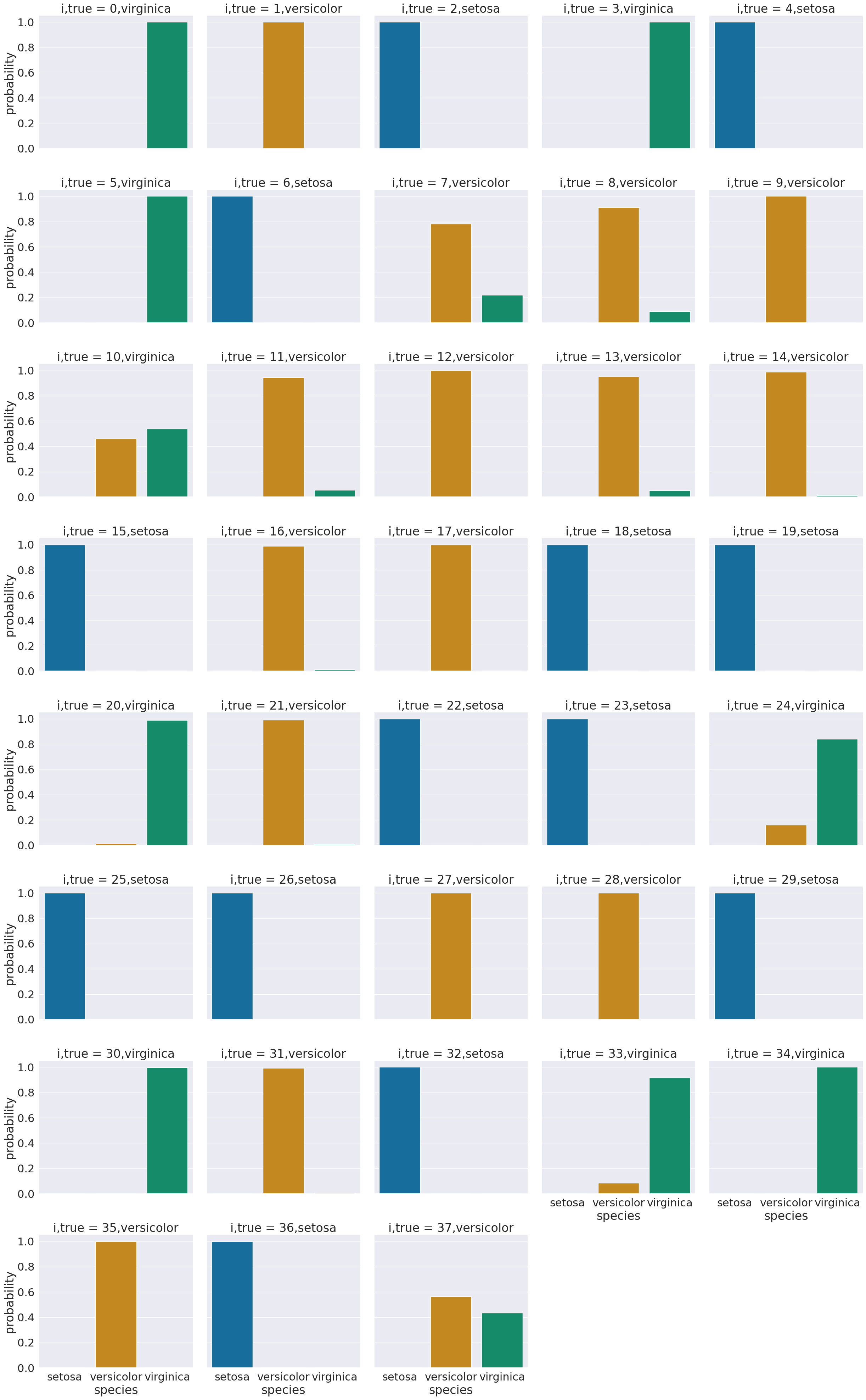
We see that most sampples have nearly all of their probability mass (all probabiilties in a distribution sum (or integrate if continuous) to 1, but a few samples are not.

17.2. Questions After Class

17.2.1. What are the train and test datasets?

They are subsets of the original dataset.

For example if I use the index of the test set to pick a set of rows from the original dataset

iris_df.iloc[X_test.index[:5]]

	sepal_length	sepal_width	petal_length	petal_width	species
114	5.8	2.8	5.1	2.4	virginica
62	6.0	2.2	4.0	1.0	versicolor
33	5.5	4.2	1.4	0.2	setosa
107	7.3	2.9	6.3	1.8	virginica
7	5.0	3.4	1.5	0.2	setosa

and compare it to the actual test set

X_test.head()

	petal_width	sepal_length	sepal_width	petal_length
114	2.4	5.8	2.8	5.1
62	1.0	6.0	2.2	4.0
33	0.2	5.5	4.2	1.4
107	1.8	7.3	2.9	6.3
7	0.2	5.0	3.4	1.5

the columns are out of order because of how we created the train test splits, but the data are the same.

We split the data so that we can be sure that the algorithm is generalizing what it learned from the test set.

17.2.2. y_pred = gnb.predict(X_test). What is this predicting?

This uses the model to find the highest probability class for each sample in the test set.

17.2.3. What is the best number of samples to use to have the most accurate predictions?

That will vary and is one of the things you will experiment with in assignment 7.

17.2.4. need more clarification on the confusion_matrix. not sure what its doing if we already proved y_pred and y_test are the same

In this case, it does basically repeat that, except it does it per species (class). Notice that all of the numbers are on the diagonal of the matrix.

17.2.5. Can we use this machine learning to predict MIC data of peptides based off their sequences and similarly output data for new synthetic AMPS?

Possibly, but maybe a different model. I would need to know more about the dat here and I am not a biologist. We can discuss this in office hours.

17.2.6. If more samples of data increases accuracy of the model, is there ever a point where adding more samples of data does not increase accuracy?

More samples increases the reliability of the estimate, and generally increases the accuracy, but not always. We will see different ways that more data does not increase over the next few weeks. You will also experiment with this in your next assignment (I give you the steps, you interpret the results)