Learning Curves
Contents
35. Learning Curves#
import matplotlib.pyplot as plt
import numpy as np
import seaborn as sns
import pandas as pd
from sklearn import datasets
from sklearn import cluster

from sklearn import naive_bayes
from sklearn import svm
from sklearn import tree
# import the whole model selection module
from sklearn import model_selection
sns.set_theme(palette='colorblind')
35.1. Digits Dataset#
Today, we’ll load a new dataset and use the default sklearn data structure for datasets. We get back the default data stucture when we use a load_ function without any parameters at all.
digits = datasets.load_digits()
This shows us that the type is defined by sklearn and they called it bunch:
type(digits)
sklearn.utils._bunch.Bunch
We can print it out to begin exploring it.
digits
{'data': array([[ 0.,  0.,  5., ...,  0.,  0.,  0.],
        [ 0.,  0.,  0., ..., 10.,  0.,  0.],
        [ 0.,  0.,  0., ..., 16.,  9.,  0.],
        ...,
        [ 0.,  0.,  1., ...,  6.,  0.,  0.],
        [ 0.,  0.,  2., ..., 12.,  0.,  0.],
        [ 0.,  0., 10., ..., 12.,  1.,  0.]]),
 'target': array([0, 1, 2, ..., 8, 9, 8]),
 'frame': None,
 'feature_names': ['pixel_0_0',
  'pixel_0_1',
  'pixel_0_2',
  'pixel_0_3',
  'pixel_0_4',
  'pixel_0_5',
  'pixel_0_6',
  'pixel_0_7',
  'pixel_1_0',
  'pixel_1_1',
  'pixel_1_2',
  'pixel_1_3',
  'pixel_1_4',
  'pixel_1_5',
  'pixel_1_6',
  'pixel_1_7',
  'pixel_2_0',
  'pixel_2_1',
  'pixel_2_2',
  'pixel_2_3',
  'pixel_2_4',
  'pixel_2_5',
  'pixel_2_6',
  'pixel_2_7',
  'pixel_3_0',
  'pixel_3_1',
  'pixel_3_2',
  'pixel_3_3',
  'pixel_3_4',
  'pixel_3_5',
  'pixel_3_6',
  'pixel_3_7',
  'pixel_4_0',
  'pixel_4_1',
  'pixel_4_2',
  'pixel_4_3',
  'pixel_4_4',
  'pixel_4_5',
  'pixel_4_6',
  'pixel_4_7',
  'pixel_5_0',
  'pixel_5_1',
  'pixel_5_2',
  'pixel_5_3',
  'pixel_5_4',
  'pixel_5_5',
  'pixel_5_6',
  'pixel_5_7',
  'pixel_6_0',
  'pixel_6_1',
  'pixel_6_2',
  'pixel_6_3',
  'pixel_6_4',
  'pixel_6_5',
  'pixel_6_6',
  'pixel_6_7',
  'pixel_7_0',
  'pixel_7_1',
  'pixel_7_2',
  'pixel_7_3',
  'pixel_7_4',
  'pixel_7_5',
  'pixel_7_6',
  'pixel_7_7'],
 'target_names': array([0, 1, 2, 3, 4, 5, 6, 7, 8, 9]),
 'images': array([[[ 0.,  0.,  5., ...,  1.,  0.,  0.],
         [ 0.,  0., 13., ..., 15.,  5.,  0.],
         [ 0.,  3., 15., ..., 11.,  8.,  0.],
         ...,
         [ 0.,  4., 11., ..., 12.,  7.,  0.],
         [ 0.,  2., 14., ..., 12.,  0.,  0.],
         [ 0.,  0.,  6., ...,  0.,  0.,  0.]],

        [[ 0.,  0.,  0., ...,  5.,  0.,  0.],
         [ 0.,  0.,  0., ...,  9.,  0.,  0.],
         [ 0.,  0.,  3., ...,  6.,  0.,  0.],
         ...,
         [ 0.,  0.,  1., ...,  6.,  0.,  0.],
         [ 0.,  0.,  1., ...,  6.,  0.,  0.],
         [ 0.,  0.,  0., ..., 10.,  0.,  0.]],

        [[ 0.,  0.,  0., ..., 12.,  0.,  0.],
         [ 0.,  0.,  3., ..., 14.,  0.,  0.],
         [ 0.,  0.,  8., ..., 16.,  0.,  0.],
         ...,
         [ 0.,  9., 16., ...,  0.,  0.,  0.],
         [ 0.,  3., 13., ..., 11.,  5.,  0.],
         [ 0.,  0.,  0., ..., 16.,  9.,  0.]],

        ...,

        [[ 0.,  0.,  1., ...,  1.,  0.,  0.],
         [ 0.,  0., 13., ...,  2.,  1.,  0.],
         [ 0.,  0., 16., ..., 16.,  5.,  0.],
         ...,
         [ 0.,  0., 16., ..., 15.,  0.,  0.],
         [ 0.,  0., 15., ..., 16.,  0.,  0.],
         [ 0.,  0.,  2., ...,  6.,  0.,  0.]],

        [[ 0.,  0.,  2., ...,  0.,  0.,  0.],
         [ 0.,  0., 14., ..., 15.,  1.,  0.],
         [ 0.,  4., 16., ..., 16.,  7.,  0.],
         ...,
         [ 0.,  0.,  0., ..., 16.,  2.,  0.],
         [ 0.,  0.,  4., ..., 16.,  2.,  0.],
         [ 0.,  0.,  5., ..., 12.,  0.,  0.]],

        [[ 0.,  0., 10., ...,  1.,  0.,  0.],
         [ 0.,  2., 16., ...,  1.,  0.,  0.],
         [ 0.,  0., 15., ..., 15.,  0.,  0.],
         ...,
         [ 0.,  4., 16., ..., 16.,  6.,  0.],
         [ 0.,  8., 16., ..., 16.,  8.,  0.],
         [ 0.,  1.,  8., ..., 12.,  1.,  0.]]]),
 'DESCR': ".. _digits_dataset:\n\nOptical recognition of handwritten digits dataset\n--------------------------------------------------\n\n**Data Set Characteristics:**\n\n    :Number of Instances: 1797\n    :Number of Attributes: 64\n    :Attribute Information: 8x8 image of integer pixels in the range 0..16.\n    :Missing Attribute Values: None\n    :Creator: E. Alpaydin (alpaydin '@' boun.edu.tr)\n    :Date: July; 1998\n\nThis is a copy of the test set of the UCI ML hand-written digits datasets\nhttps://archive.ics.uci.edu/ml/datasets/Optical+Recognition+of+Handwritten+Digits\n\nThe data set contains images of hand-written digits: 10 classes where\neach class refers to a digit.\n\nPreprocessing programs made available by NIST were used to extract\nnormalized bitmaps of handwritten digits from a preprinted form. From a\ntotal of 43 people, 30 contributed to the training set and different 13\nto the test set. 32x32 bitmaps are divided into nonoverlapping blocks of\n4x4 and the number of on pixels are counted in each block. This generates\nan input matrix of 8x8 where each element is an integer in the range\n0..16. This reduces dimensionality and gives invariance to small\ndistortions.\n\nFor info on NIST preprocessing routines, see M. D. Garris, J. L. Blue, G.\nT. Candela, D. L. Dimmick, J. Geist, P. J. Grother, S. A. Janet, and C.\nL. Wilson, NIST Form-Based Handprint Recognition System, NISTIR 5469,\n1994.\n\n.. topic:: References\n\n  - C. Kaynak (1995) Methods of Combining Multiple Classifiers and Their\n    Applications to Handwritten Digit Recognition, MSc Thesis, Institute of\n    Graduate Studies in Science and Engineering, Bogazici University.\n  - E. Alpaydin, C. Kaynak (1998) Cascading Classifiers, Kybernetika.\n  - Ken Tang and Ponnuthurai N. Suganthan and Xi Yao and A. Kai Qin.\n    Linear dimensionalityreduction using relevance weighted LDA. School of\n    Electrical and Electronic Engineering Nanyang Technological University.\n    2005.\n  - Claudio Gentile. A New Approximate Maximal Margin Classification\n    Algorithm. NIPS. 2000.\n"}
We note that it has key value pairs, and that the last one is called DESCR and is text that describes the data. If we send that to the print function it will be formatted more readably.
print(digits['DESCR'])
.. _digits_dataset:

Optical recognition of handwritten digits dataset
--------------------------------------------------

**Data Set Characteristics:**

    :Number of Instances: 1797
    :Number of Attributes: 64
    :Attribute Information: 8x8 image of integer pixels in the range 0..16.
    :Missing Attribute Values: None
    :Creator: E. Alpaydin (alpaydin '@' boun.edu.tr)
    :Date: July; 1998

This is a copy of the test set of the UCI ML hand-written digits datasets
https://archive.ics.uci.edu/ml/datasets/Optical+Recognition+of+Handwritten+Digits

The data set contains images of hand-written digits: 10 classes where
each class refers to a digit.

Preprocessing programs made available by NIST were used to extract
normalized bitmaps of handwritten digits from a preprinted form. From a
total of 43 people, 30 contributed to the training set and different 13
to the test set. 32x32 bitmaps are divided into nonoverlapping blocks of
4x4 and the number of on pixels are counted in each block. This generates
an input matrix of 8x8 where each element is an integer in the range
0..16. This reduces dimensionality and gives invariance to small
distortions.

For info on NIST preprocessing routines, see M. D. Garris, J. L. Blue, G.
T. Candela, D. L. Dimmick, J. Geist, P. J. Grother, S. A. Janet, and C.
L. Wilson, NIST Form-Based Handprint Recognition System, NISTIR 5469,
1994.

.. topic:: References

  - C. Kaynak (1995) Methods of Combining Multiple Classifiers and Their
    Applications to Handwritten Digit Recognition, MSc Thesis, Institute of
    Graduate Studies in Science and Engineering, Bogazici University.
  - E. Alpaydin, C. Kaynak (1998) Cascading Classifiers, Kybernetika.
  - Ken Tang and Ponnuthurai N. Suganthan and Xi Yao and A. Kai Qin.
    Linear dimensionalityreduction using relevance weighted LDA. School of
    Electrical and Electronic Engineering Nanyang Technological University.
    2005.
  - Claudio Gentile. A New Approximate Maximal Margin Classification
    Algorithm. NIPS. 2000.
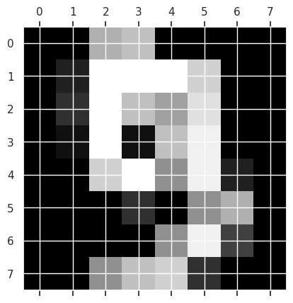
This tells us that we are going to be predicting what digit (0,1,2,3,4,5,6,7,8, or 9) is in the image.
To get an idea of what the images look like, we can use matshow which is short for matrix show. It takes a 2D matrix and plots it as a grayscale image. To get the actual color bar, we use the matplotlib plt.gray().
plt.gray()
plt.matshow(digits.images[9])
<matplotlib.image.AxesImage at 0x7efdd63370a0>
<Figure size 640x480 with 0 Axes>
35.2. Setting up the Problem#
digits_X = digits.data
digits_y = digits.target
bunch objects are designed for machine learning, so they have the features as “data” and target explicitly identified.
digits_X.shape, digits_y.shape
((1797, 64), (1797,))
This has one row for each sample and has reshaped the 8x8 image into a 64 length vector. So we have one ‘feature’ for each pixel in the images.
The size of the .images is the total number of pixel values.
1797*8*8
115008
35.3. Learning Curves#
We are going to do some model comparison, so we will instantiate estimator objects for two different classifiers.
svm_clf = svm.SVC(gamma=0.001)
gnb_clf = naive_bayes.GaussianNB()
We’re going to use a ShuffleSplit object to do Cross validation with 100 iterations to get smoother mean test and train score curves, each time with 20% data randomly selected as a validation set.
Further Reading
You can see visualization of different cross validation types in the sklearn documentation.
cv = model_selection.ShuffleSplit(n_splits=100, test_size=0.2, random_state=0)
Note
This object has a random_state object, the GridSearchCV that we were using didn’t have a way to control the random state directly, but it accepts not only integers, but also cross validation objects to the cv parameter. The KFold cross validation object also has that parameter, so we could repeat what we did in previous classes by creating a KFold object with a fixed random state.
We’ll also create a linearly spaced list of training percentages.
Important
You could speed it up by splitting it into jobs with the n_jobs parameter
Now we can create the learning curve.
train_sizes = np.linspace(.05,1,10)

train_sizes_svm, train_scores_svm, test_scores_svm, fit_times_svm, score_times_svm = model_selection.learning_curve(
    svm_clf,
    digits_X,
    digits_y,
    cv=cv,
    train_sizes=train_sizes,
    return_times=True,)
---------------------------------------------------------------------------
KeyboardInterrupt                         Traceback (most recent call last)
Cell In[12], line 3
      1 train_sizes = np.linspace(.05,1,10)
----> 3 train_sizes_svm, train_scores_svm, test_scores_svm, fit_times_svm, score_times_svm = model_selection.learning_curve(
      4     svm_clf,
      5     digits_X,
      6     digits_y,
      7     cv=cv,
      8     train_sizes=train_sizes,
      9     return_times=True,)

File /opt/hostedtoolcache/Python/3.9.16/x64/lib/python3.9/site-packages/sklearn/model_selection/_validation.py:1579, in learning_curve(estimator, X, y, groups, train_sizes, cv, scoring, exploit_incremental_learning, n_jobs, pre_dispatch, verbose, shuffle, random_state, error_score, return_times, fit_params)
   1576     for n_train_samples in train_sizes_abs:
   1577         train_test_proportions.append((train[:n_train_samples], test))
-> 1579 results = parallel(
   1580     delayed(_fit_and_score)(
   1581         clone(estimator),
   1582         X,
   1583         y,
   1584         scorer,
   1585         train,
   1586         test,
   1587         verbose,
   1588         parameters=None,
   1589         fit_params=fit_params,
   1590         return_train_score=True,
   1591         error_score=error_score,
   1592         return_times=return_times,
   1593     )
   1594     for train, test in train_test_proportions
   1595 )
   1596 results = _aggregate_score_dicts(results)
   1597 train_scores = results["train_scores"].reshape(-1, n_unique_ticks).T

File /opt/hostedtoolcache/Python/3.9.16/x64/lib/python3.9/site-packages/joblib/parallel.py:1088, in Parallel.__call__(self, iterable)
   1085 if self.dispatch_one_batch(iterator):
   1086     self._iterating = self._original_iterator is not None
-> 1088 while self.dispatch_one_batch(iterator):
   1089     pass
   1091 if pre_dispatch == "all" or n_jobs == 1:
   1092     # The iterable was consumed all at once by the above for loop.
   1093     # No need to wait for async callbacks to trigger to
   1094     # consumption.

File /opt/hostedtoolcache/Python/3.9.16/x64/lib/python3.9/site-packages/joblib/parallel.py:901, in Parallel.dispatch_one_batch(self, iterator)
    899     return False
    900 else:
--> 901     self._dispatch(tasks)
    902     return True

File /opt/hostedtoolcache/Python/3.9.16/x64/lib/python3.9/site-packages/joblib/parallel.py:819, in Parallel._dispatch(self, batch)
    817 with self._lock:
    818     job_idx = len(self._jobs)
--> 819     job = self._backend.apply_async(batch, callback=cb)
    820     # A job can complete so quickly than its callback is
    821     # called before we get here, causing self._jobs to
    822     # grow. To ensure correct results ordering, .insert is
    823     # used (rather than .append) in the following line
    824     self._jobs.insert(job_idx, job)

File /opt/hostedtoolcache/Python/3.9.16/x64/lib/python3.9/site-packages/joblib/_parallel_backends.py:208, in SequentialBackend.apply_async(self, func, callback)
    206 def apply_async(self, func, callback=None):
    207     """Schedule a func to be run"""
--> 208     result = ImmediateResult(func)
    209     if callback:
    210         callback(result)

File /opt/hostedtoolcache/Python/3.9.16/x64/lib/python3.9/site-packages/joblib/_parallel_backends.py:597, in ImmediateResult.__init__(self, batch)
    594 def __init__(self, batch):
    595     # Don't delay the application, to avoid keeping the input
    596     # arguments in memory
--> 597     self.results = batch()

File /opt/hostedtoolcache/Python/3.9.16/x64/lib/python3.9/site-packages/joblib/parallel.py:288, in BatchedCalls.__call__(self)
    284 def __call__(self):
    285     # Set the default nested backend to self._backend but do not set the
    286     # change the default number of processes to -1
    287     with parallel_backend(self._backend, n_jobs=self._n_jobs):
--> 288         return [func(*args, **kwargs)
    289                 for func, args, kwargs in self.items]

File /opt/hostedtoolcache/Python/3.9.16/x64/lib/python3.9/site-packages/joblib/parallel.py:288, in <listcomp>(.0)
    284 def __call__(self):
    285     # Set the default nested backend to self._backend but do not set the
    286     # change the default number of processes to -1
    287     with parallel_backend(self._backend, n_jobs=self._n_jobs):
--> 288         return [func(*args, **kwargs)
    289                 for func, args, kwargs in self.items]

File /opt/hostedtoolcache/Python/3.9.16/x64/lib/python3.9/site-packages/sklearn/utils/fixes.py:117, in _FuncWrapper.__call__(self, *args, **kwargs)
    115 def __call__(self, *args, **kwargs):
    116     with config_context(**self.config):
--> 117         return self.function(*args, **kwargs)

File /opt/hostedtoolcache/Python/3.9.16/x64/lib/python3.9/site-packages/sklearn/model_selection/_validation.py:686, in _fit_and_score(estimator, X, y, scorer, train, test, verbose, parameters, fit_params, return_train_score, return_parameters, return_n_test_samples, return_times, return_estimator, split_progress, candidate_progress, error_score)
    684         estimator.fit(X_train, **fit_params)
    685     else:
--> 686         estimator.fit(X_train, y_train, **fit_params)
    688 except Exception:
    689     # Note fit time as time until error
    690     fit_time = time.time() - start_time

File /opt/hostedtoolcache/Python/3.9.16/x64/lib/python3.9/site-packages/sklearn/svm/_base.py:252, in BaseLibSVM.fit(self, X, y, sample_weight)
    249     print("[LibSVM]", end="")
    251 seed = rnd.randint(np.iinfo("i").max)
--> 252 fit(X, y, sample_weight, solver_type, kernel, random_seed=seed)
    253 # see comment on the other call to np.iinfo in this file
    255 self.shape_fit_ = X.shape if hasattr(X, "shape") else (n_samples,)

File /opt/hostedtoolcache/Python/3.9.16/x64/lib/python3.9/site-packages/sklearn/svm/_base.py:331, in BaseLibSVM._dense_fit(self, X, y, sample_weight, solver_type, kernel, random_seed)
    317 libsvm.set_verbosity_wrap(self.verbose)
    319 # we don't pass **self.get_params() to allow subclasses to
    320 # add other parameters to __init__
    321 (
    322     self.support_,
    323     self.support_vectors_,
    324     self._n_support,
    325     self.dual_coef_,
    326     self.intercept_,
    327     self._probA,
    328     self._probB,
    329     self.fit_status_,
    330     self._num_iter,
--> 331 ) = libsvm.fit(
    332     X,
    333     y,
    334     svm_type=solver_type,
    335     sample_weight=sample_weight,
    336     # TODO(1.4): Replace "_class_weight" with "class_weight_"
    337     class_weight=getattr(self, "_class_weight", np.empty(0)),
    338     kernel=kernel,
    339     C=self.C,
    340     nu=self.nu,
    341     probability=self.probability,
    342     degree=self.degree,
    343     shrinking=self.shrinking,
    344     tol=self.tol,
    345     cache_size=self.cache_size,
    346     coef0=self.coef0,
    347     gamma=self._gamma,
    348     epsilon=self.epsilon,
    349     max_iter=self.max_iter,
    350     random_seed=random_seed,
    351 )
    353 self._warn_from_fit_status()

KeyboardInterrupt:
It returns the list of the counts for each training size (we input percentages and it returns counts)
train_sizes_svm
The other parameters, it returns a list for each length that’s 100 long because our cross validation was 100 iterations.
fit_times_svm.shape
We can save it in a DataFrame after averaging over the 100 trials.
svm_learning_df = pd.DataFrame(data = train_sizes_svm, columns = ['train_size'])
# svm_learning_df['train_size'] = train_sizes_svm
svm_learning_df['train_score'] = np.mean(train_scores_svm,axis=1)
svm_learning_df['test_score'] = np.mean(test_scores_svm,axis=1)
svm_learning_df['fit_time'] = np.mean(fit_times_svm,axis=1)
svm_learning_df['score_times'] = np.mean(score_times_svm,axis=1)
svm_learning_df.head()
We can use our skills in transforming data to make it easier to exmine just a subset of the scores.
svm_learning_df_scores = svm_learning_df.melt(id_vars=['train_size'],
                                                value_vars=['train_score','test_score'])
svm_learning_df_scores.head(2)
This new DataFrame allows us to make convenient plots.
sns.lineplot(data=svm_learning_df_scores,x='train_size',y='value',hue='variable')
35.3.1. Gaussian Naive Bayes#
We can do the same thing with GNB
train_sizes_gnb, train_scores_gnb, test_scores_gnb, fit_times_gnb, score_times_gnb = model_selection.learning_curve(
  gnb_clf,
  digits_X,
  digits_y,
  cv=cv,
  train_sizes=train_sizes,
  return_times=True,)
gnb_learning_df = pd.DataFrame(data = train_sizes_gnb, columns = ['train_size'])
# gnb_learning_df['train_size'] = train_sizes_gnb
gnb_learning_df['train_score'] = np.mean(train_scores_gnb,axis=1)
gnb_learning_df['test_score'] = np.mean(test_scores_gnb,axis=1)
gnb_learning_df['fit_time'] = np.mean(fit_times_gnb,axis=1)
gnb_learning_df['score_times_gnb'] = np.mean(score_times_gnb,axis=1)
gnb_learning_scores = gnb_learning_df.melt(id_vars=['train_size'],value_vars=['train_score','test_score'])
sns.lineplot(data = gnb_learning_scores, x ='train_size', y='value',hue='variable')
Notice in this case that the training accuracy starts high with the test accuracy low. This big gap means that the model was overfitting to something that was different about the training set from the test set. It was
35.4. Questions After Class#
35.4.1. how do I run the code to pull issues?#
This uses the GitHub CLI
gh issue list --state all -L 45 --json title,url,state > grade-tracker.json
35.4.2. Is fit time as important as accuracy? I would think generally for real life application we would want results over time.#
Fit time is generally not as important as accuracy when deploying a model. This question gets at a really important point. Some of the metrics that we have for machine learning algorithms are for evaluating the learning algorithm, if someone develops a new learning algorithm that can perform as well as old ones, but faster that’s really helpful. You are correct,
That said, the score time can be really important in a deployed model.
35.4.3. Why in the SVC model did we used gamma=0.001 and not other values? Why does that parameter represent in the model?#
The gamma \(\gamma\) parameter for the default rbf kernel controls basically how wavy the line is. I set it to a value that is known to work well for this dataset because, for time reasons, I did not want to also do a grid search.
35.4.4. I’m sure it will be in the notes but a better understanding of how learning curve works#
35.4.5. Can you go over the melt function again?#
• running code will be posted tonight correct?
• nothing at the moment