
Intro to Data Cleaning
Contents
8. Intro to Data Cleaning#
This week, we’ll be cleaning data.
Cleaning data is labor intensive and requires making subjective choices.
We’ll focus on, and assess you on, manipulating data correctly, making reasonable
choices, and documenting the choices you make carefully.
We’ll focus on the programming tools that get used in cleaning data in class this week:
reshaping data
handling missing or incorrect values
renaming columns
import pandas as pd
import seaborn as sns

# sns.set_theme(pallete='colorblind')
8.1. Tidy Data#
Read in the three csv files described below and store them in a list of dataFrames
url_base = 'https://raw.githubusercontent.com/rhodyprog4ds/rhodyds/main/data/'

datasets = ['study_a.csv','study_b.csv','study_c.csv']
df_list = [pd.read_csv(url_base + current) for current in datasets]
type(df_list)
list
type(df_list[0])
pandas.core.frame.DataFrame
df_list[0]
| name | treatmenta | treatmentb | |
|---|---|---|---|
| 0 | John Smith | - | 2 |
| 1 | Jane Doe | 16 | 11 |
| 2 | Mary Johnson | 3 | 1 |
df_list[1]
| intervention | John Smith | Jane Doe | Mary Johnson | |
|---|---|---|---|---|
| 0 | treatmenta | - | 16 | 3 |
| 1 | treatmentb | 2 | 11 | 1 |
df_list[2]
| person | treatment | result | |
|---|---|---|---|
| 0 | John Smith | a | - |
| 1 | Jane Doe | a | 16 |
| 2 | Mary Johnson | a | 3 |
| 3 | John Smith | b | 2 |
| 4 | Jane Doe | b | 11 |
| 5 | Mary Johnson | b | 1 |
These three all show the same data, but let’s say we have two goals:
find the average effect per person across treatments
find the average effect per treatment across people
This works differently for these three versions.
df_list[0].mean()
/tmp/ipykernel_2091/2274987639.py:1: FutureWarning: The default value of numeric_only in DataFrame.mean is deprecated. In a future version, it will default to False. In addition, specifying 'numeric_only=None' is deprecated. Select only valid columns or specify the value of numeric_only to silence this warning.
  df_list[0].mean()
treatmenta   -54.333333
treatmentb     4.666667
dtype: float64
we get the average per treatment, but to get the average per person, we have to go across rows, which we can do here, but doesn’t work as well with plotting
df_list[0].mean(axis=1)
/tmp/ipykernel_2091/1371725361.py:1: FutureWarning: Dropping of nuisance columns in DataFrame reductions (with 'numeric_only=None') is deprecated; in a future version this will raise TypeError.  Select only valid columns before calling the reduction.
  df_list[0].mean(axis=1)
0     2.0
1    11.0
2     1.0
dtype: float64
and this is not well labeled.
Let’s try the next one.
df_list[1].mean()
/tmp/ipykernel_2091/1105758803.py:1: FutureWarning: The default value of numeric_only in DataFrame.mean is deprecated. In a future version, it will default to False. In addition, specifying 'numeric_only=None' is deprecated. Select only valid columns or specify the value of numeric_only to silence this warning.
  df_list[1].mean()
John Smith      -1.0
Jane Doe        13.5
Mary Johnson     2.0
dtype: float64
Now we get the average per person, but what about per treatment? again we have to go across rows instead.
df_list[1].mean(axis=1)
/tmp/ipykernel_2091/1112167831.py:1: FutureWarning: Dropping of nuisance columns in DataFrame reductions (with 'numeric_only=None') is deprecated; in a future version this will raise TypeError.  Select only valid columns before calling the reduction.
  df_list[1].mean(axis=1)
0    9.5
1    6.0
dtype: float64
For the third one, however, we can use groupby
df_list[2].groupby('person').mean()
/tmp/ipykernel_2091/906930014.py:1: FutureWarning: The default value of numeric_only in DataFrameGroupBy.mean is deprecated. In a future version, numeric_only will default to False. Either specify numeric_only or select only columns which should be valid for the function.
  df_list[2].groupby('person').mean()
| result | |
|---|---|
| person | |
| Jane Doe | 805.5 |
| John Smith | -1.0 |
| Mary Johnson | 15.5 |
df_list[2].groupby('treatment').mean()
/tmp/ipykernel_2091/2480310521.py:1: FutureWarning: The default value of numeric_only in DataFrameGroupBy.mean is deprecated. In a future version, numeric_only will default to False. Either specify numeric_only or select only columns which should be valid for the function.
  df_list[2].groupby('treatment').mean()
| result | |
|---|---|
| treatment | |
| a | -54.333333 |
| b | 703.666667 |
The original Tidy Data paper is worth reading to build a deeper understanding of these ideas.
8.2. Tidying Data#
Let’s reshape the first one to match the tidy one. First, we will save it to a DataFrame, this makes things easier to read and enables us to use the built in help in jupyter, because it can’t check types too many levels into a data structure.
treat_df = df_list[0]
Let’s look at it again, so we can see
treat_df.head()
| name | treatmenta | treatmentb | |
|---|---|---|---|
| 0 | John Smith | - | 2 |
| 1 | Jane Doe | 16 | 11 |
| 2 | Mary Johnson | 3 | 1 |
df_list[0].columns
Index(['name', 'treatmenta', 'treatmentb'], dtype='object')
df_a = df_list[0]
df_a.melt(id_vars=['name'],value_vars=['treatmenta','treatmentb'],
          value_name='result',var_name='treatment')
| name | treatment | result | |
|---|---|---|---|
| 0 | John Smith | treatmenta | - |
| 1 | Jane Doe | treatmenta | 16 |
| 2 | Mary Johnson | treatmenta | 3 |
| 3 | John Smith | treatmentb | 2 |
| 4 | Jane Doe | treatmentb | 11 |
| 5 | Mary Johnson | treatmentb | 1 |
When we melt a dataset:
the
id_varsstay as columnsthe data from the
value_varscolumns become the values in thevaluecolumnthe column names from the
value_varsbecome the values in thevariablecolumnwe can rename the value and the variable columns.
Let’s do it for our coffee data:
arabica_data_url = 'https://raw.githubusercontent.com/jldbc/coffee-quality-database/master/data/arabica_data_cleaned.csv'
coffee_df = pd.read_csv(arabica_data_url)
scores_of_interest = ['Balance','Aroma','Body','Aftertaste']
coffee_tall = coffee_df.melt(id_vars=['Country.of.Origin','Color'],
                             value_vars=scores_of_interest
               ,var_name = 'Score')
coffee_tall.head()
| Country.of.Origin | Color | Score | value | |
|---|---|---|---|---|
| 0 | Ethiopia | Green | Balance | 8.42 |
| 1 | Ethiopia | Green | Balance | 8.42 |
| 2 | Guatemala | NaN | Balance | 8.42 |
| 3 | Ethiopia | Green | Balance | 8.25 |
| 4 | Ethiopia | Green | Balance | 8.33 |
Notice that the actual column names inside the scores_of_interest variable become the values in the variable column.
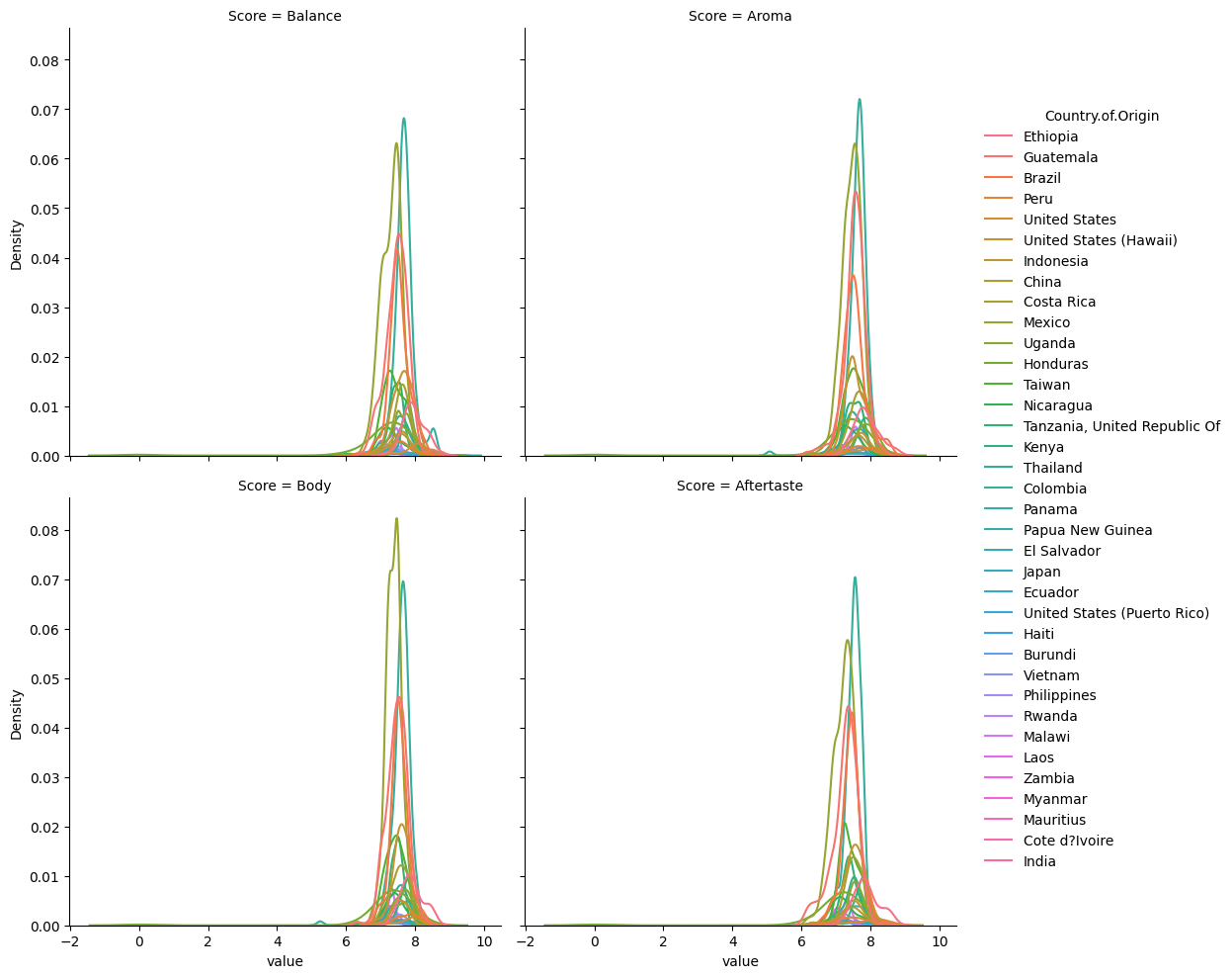
This one we can plot in more ways:
sns.displot(data=coffee_tall, x='value',hue='Country.of.Origin',
            col='Score',kind='kde',col_wrap=2)
/tmp/ipykernel_2091/3603277008.py:1: UserWarning: Dataset has 0 variance; skipping density estimate. Pass `warn_singular=False` to disable this warning.
  sns.displot(data=coffee_tall, x='value',hue='Country.of.Origin',
/tmp/ipykernel_2091/3603277008.py:1: UserWarning: Dataset has 0 variance; skipping density estimate. Pass `warn_singular=False` to disable this warning.
  sns.displot(data=coffee_tall, x='value',hue='Country.of.Origin',
/tmp/ipykernel_2091/3603277008.py:1: UserWarning: Dataset has 0 variance; skipping density estimate. Pass `warn_singular=False` to disable this warning.
  sns.displot(data=coffee_tall, x='value',hue='Country.of.Origin',
/tmp/ipykernel_2091/3603277008.py:1: UserWarning: Dataset has 0 variance; skipping density estimate. Pass `warn_singular=False` to disable this warning.
  sns.displot(data=coffee_tall, x='value',hue='Country.of.Origin',
/tmp/ipykernel_2091/3603277008.py:1: UserWarning: Dataset has 0 variance; skipping density estimate. Pass `warn_singular=False` to disable this warning.
  sns.displot(data=coffee_tall, x='value',hue='Country.of.Origin',
<seaborn.axisgrid.FacetGrid at 0x7fe96985ae50>
8.3. Filtering Data#
high_prod = coffee_df[coffee_df['Number.of.Bags']>250]
high_prod.shape
(368, 44)
coffee_df.shape
(1311, 44)
We see that filters and reduces. We can use any boolean expression in the square brackets.
top_balance = coffee_df[coffee_df['Balance']>coffee_df['Balance'].quantile(.75)]
top_balance.shape
(252, 44)
We can confirm that we got only the top 25% of balance scores:
top_balance.describe()
| Unnamed: 0 | Number.of.Bags | Aroma | Flavor | Aftertaste | Acidity | Body | Balance | Uniformity | Clean.Cup | Sweetness | Cupper.Points | Total.Cup.Points | Moisture | Category.One.Defects | Quakers | Category.Two.Defects | altitude_low_meters | altitude_high_meters | altitude_mean_meters | |
|---|---|---|---|---|---|---|---|---|---|---|---|---|---|---|---|---|---|---|---|---|
| count | 252.000000 | 252.000000 | 252.000000 | 252.000000 | 252.000000 | 252.000000 | 252.000000 | 252.000000 | 252.000000 | 252.000000 | 252.000000 | 252.000000 | 252.00000 | 252.000000 | 252.000000 | 252.000000 | 252.000000 | 190.000000 | 190.000000 | 190.000000 |
| mean | 273.535714 | 153.337302 | 7.808889 | 7.837659 | 7.734167 | 7.824881 | 7.780159 | 8.003095 | 9.885278 | 9.896667 | 9.885952 | 7.865714 | 84.52504 | 0.072579 | 0.361111 | 0.150794 | 2.801587 | 1343.138168 | 1424.547053 | 1383.842611 |
| std | 284.249040 | 126.498576 | 0.355319 | 0.318172 | 0.302481 | 0.320253 | 0.317712 | 0.213056 | 0.363303 | 0.470514 | 0.380433 | 0.383738 | 1.91563 | 0.051682 | 1.249923 | 0.692216 | 4.659771 | 480.927004 | 503.063351 | 484.286247 |
| min | 1.000000 | 0.000000 | 5.080000 | 7.170000 | 6.920000 | 7.080000 | 5.250000 | 7.830000 | 6.670000 | 5.330000 | 6.670000 | 5.170000 | 77.00000 | 0.000000 | 0.000000 | 0.000000 | 0.000000 | 1.000000 | 1.000000 | 1.000000 |
| 25% | 65.750000 | 12.750000 | 7.647500 | 7.670000 | 7.500000 | 7.670000 | 7.670000 | 7.830000 | 10.000000 | 10.000000 | 10.000000 | 7.670000 | 83.42000 | 0.000000 | 0.000000 | 0.000000 | 0.000000 | 1162.500000 | 1200.000000 | 1200.000000 |
| 50% | 171.500000 | 165.500000 | 7.780000 | 7.830000 | 7.750000 | 7.830000 | 7.750000 | 7.920000 | 10.000000 | 10.000000 | 10.000000 | 7.830000 | 84.46000 | 0.100000 | 0.000000 | 0.000000 | 1.000000 | 1400.000000 | 1500.000000 | 1450.000000 |
| 75% | 378.250000 | 275.000000 | 8.000000 | 8.000000 | 7.920000 | 8.000000 | 7.920000 | 8.080000 | 10.000000 | 10.000000 | 10.000000 | 8.080000 | 85.52000 | 0.110000 | 0.000000 | 0.000000 | 3.000000 | 1695.000000 | 1800.000000 | 1750.000000 |
| max | 1260.000000 | 360.000000 | 8.750000 | 8.830000 | 8.670000 | 8.750000 | 8.580000 | 8.750000 | 10.000000 | 10.000000 | 10.000000 | 9.250000 | 90.58000 | 0.210000 | 10.000000 | 6.000000 | 40.000000 | 2560.000000 | 2560.000000 | 2560.000000 |
We can also use the isin method to filter by comparing to an iterable type
total_per_country = coffee_df.groupby('Country.of.Origin')['Number.of.Bags'].sum()
top_countries = total_per_country.sort_values(ascending=False)[:10].index
top_coffee_df = coffee_df[coffee_df['Country.of.Origin'].isin(top_countries)]
8.4. Questions after class#
8.4.1. In the data we had about treatment a and treatment b. Say there was another column that provided information about the age of the people. Could we create another value variable to or would we put it in the value_vars list along with treatment a and treatmentb?#
We can have multiple variables as the id_vars so that the dataset would have 4 columns instead of 3.
8.4.2. Can we clean data within any row of the data as long as there is a column name for it?#
Yes
8.4.3. How to clean larger datasets#
Everything we will learn will work in any context that you can load the dataset into RAM on the computer you are working on; or process it in batches.
8.4.4. with very large data sets, how can you tell id there are missing values or incorrect types present?#
We use ways of checking the values, like the info method to check the whole column.
8.4.5. Are there any prebuilt methods to identify and remove extreme outliers?#
There may be, that is a good thing to look in the documentation for. However, typically the definition of an outlier is best made within context, so the filtering strategy that we just used would be the way to remove them, after doign some EDA.
8.4.6. Is there a specific metric to which a dataset must meet to consider it ‘cleaned’?#
It’s “clean” when it will work for the analysis you want to do. This means clean enough for one analysis may not be enough for another goal. Domain expertise is alwasy important.
8.4.7. Are there any packages we may utilize that help us clean data more effectively?#
8.4.8. Things we will do later this week:#
adding more data to a DataFrame in jupyter notebook?
replace values
deal with NaN values in a dataset?
8.4.9. Next week#
What is the difference between different types of merging data frames (inner, outer, left, right, etc)?